NLL training of a Gaussianization flow

00 — NLL training of a Gaussianization flow¶

Part 3 built RBIG: rotation + marginal blocks fit greedily, each layer optimised once against the data in front of it and never revisited. A parametric Gaussianization flow uses the same architecture — a stack of rotations and learnable marginal transforms — but treats every block’s parameters as free and fits them jointly, end-to-end, by maximum likelihood — the defining recipe for normalizing flows Papamakarios et al. (2021). The objective is the negative log-likelihood, and it comes straight from the change-of-variables rule (Part 0 00):

\log p_X(x) = \log p_Z\big(T_\theta(x)\big) + \log\big|\det J_{T_\theta}(x)\big|, \qquad \mathcal{L}(\theta) = -\tfrac{1}{N}\sum_i \log p_X(x_i).

((1))

What you will see

The NLL objective decomposed into its two terms — a base log-density and a log-determinant — confirmed against flow.log_prob.
A gauss_flows gaussianization_flow trained on two-moons with an optax loop using gradient clipping and a cyclic (one-cycle cosine) learning rate — enough to match a greedy RBIG fit.
Iterative vs parametric: the greedy RBIG fit of Part 3 against the end-to-end-trained flow on the same target.

import warnings

warnings.filterwarnings("ignore")

import jax
import equinox as eqx
import jax.numpy as jnp
import jax.random as jr
import matplotlib.pyplot as plt
import numpy as np
import optax
from sklearn.datasets import make_moons

import gauss_flows as gf
from _style import SCATTER_KW, style_ax

jax.config.update("jax_enable_x64", True)
rng = np.random.default_rng(0)

X, _ = make_moons(n_samples=3000, noise=0.08, random_state=0)
X = jnp.asarray((X - X.mean(0)) / X.std(0))

1. The NLL objective and its anatomy¶

A flow $T_\theta$ maps data $x$ to a latent $z = T_\theta(x)$ with base distribution $p_Z = \mathcal{N}(0,I)$ . Its log-density at $x$ has two parts: the base log-density of where $x$ lands, $\log p_Z(z)$ , and the log-determinant $\log|\det J_{T_\theta}(x)|$ that accounts for how the map stretches volume. Training minimises the mean NLL. We build an (untrained) flow and confirm the decomposition against its log_prob.

flow0 = gf.gaussianization_flow(jr.key(0), n_dims=2, n_layers=8, n_components=8)

def nll_terms(flow, x):
    """Split log p(x) into (base log-density, log|det J|)."""
    z, log_det = flow.bijection.inverse_and_log_det(x)   # x -> z, density direction
    return flow.base_dist.log_prob(z), log_det

base, logdet = jax.vmap(lambda x: nll_terms(flow0, x))(X)
logp = jax.vmap(flow0.log_prob)(X)
print(f"mean base log p_Z(z) = {float(base.mean()):.3f}")
print(f"mean log|det J|      = {float(logdet.mean()):.3f}")
print(f"sum                  = {float((base + logdet).mean()):.3f}")
print(f"flow.log_prob mean   = {float(logp.mean()):.3f}   "
      f"(match: {bool(jnp.allclose(base + logdet, logp))})")
print(f"=> initial NLL = {-float(logp.mean()):.3f}")

mean base log p_Z(z) = -2.041
mean log|det J|      = -14.894
sum                  = -16.934
flow.log_prob mean   = -16.934   (match: True)
=> initial NLL = 16.934

The two terms sum exactly to flow.log_prob — that identity is the loss the optimiser will minimise. The base term rewards mapping data to high-density regions of $\mathcal{N}(0,I)$ ; the log-det term prevents the cheap cheat of just shrinking everything toward the origin (it penalises volume contraction). NLL training balances the two.

2. Train end-to-end with optax¶

gauss_flows ships a convenience trainer (fit_gaussianization_flow), but a Gaussianization flow is just an equinox module, so we can train it with a hand-built optax loop and add the bells and whistles that make deep flows converge: gradient clipping (clip_by_global_norm, so a rare exploding batch cannot wreck the parameters) and a cyclic learning-rate schedule (cosine_onecycle_schedule — warm up, then anneal to near zero). The loss is the NLL of §1; gradients come from eqx.filter_value_and_grad.

def train_flow(flow, X, *, steps, peak_lr, clip_norm, batch, seed=1):
    """NLL training with gradient clipping + a one-cycle cosine LR schedule."""
    params, static = eqx.partition(flow, eqx.is_inexact_array)
    schedule = optax.cosine_onecycle_schedule(transition_steps=steps, peak_value=peak_lr)
    opt = optax.chain(optax.clip_by_global_norm(clip_norm), optax.adam(schedule))
    state = opt.init(params)

    @eqx.filter_jit
    def step(params, state, xb):
        loss, grads = eqx.filter_value_and_grad(
            lambda p: -jnp.mean(jax.vmap(eqx.combine(p, static).log_prob)(xb)))(params)
        updates, state = opt.update(grads, state)
        return eqx.apply_updates(params, updates), state, loss

    key = jr.key(seed)
    losses = []
    for i in range(steps):
        key, sk = jr.split(key)
        idx = jr.randint(sk, (batch,), 0, X.shape[0])
        params, state, loss = step(params, state, X[idx])
        if i % 50 == 0:
            losses.append(float(loss))
    return eqx.combine(params, static), np.array(losses), schedule

STEPS, PEAK_LR = 3000, 3e-3
flow, losses, schedule = train_flow(flow0, X, steps=STEPS, peak_lr=PEAK_LR,
                                    clip_norm=1.0, batch=512)

logp_final = jax.vmap(flow.log_prob)(X)
z_final = jax.vmap(lambda x: flow.bijection.inverse_and_log_det(x)[0])(X)
print(f"NLL: {-float(logp.mean()):.3f} (init) -> {-float(logp_final.mean()):.3f} (trained), "
      f"{STEPS} steps")
print(f"latent z after training: mean = {float(z_final.mean()):+.3f}, std = {float(z_final.std()):.3f}")

fig, (axL, axM, axR) = plt.subplots(1, 3, figsize=(15, 4.2))
axL.plot(np.arange(len(losses)) * 50, losses, color="tab:blue", lw=2)
axL.set(title="NLL training curve", xlabel="step", ylabel="negative log-likelihood")
style_ax(axL)
axM.plot([float(schedule(i)) for i in range(STEPS)], color="tab:purple", lw=2)
axM.set(title="cyclic learning rate (one-cycle cosine)", xlabel="step", ylabel="learning rate")
style_ax(axM)
axR.scatter(z_final[:, 0], z_final[:, 1], color="tab:orange", **SCATTER_KW)
axR.set(title="latent $z = T_\\theta(x)$ (Gaussianized)", xlabel="$z_0$", ylabel="$z_1$")
axR.axhline(0, color="k", lw=0.6); axR.axvline(0, color="k", lw=0.6)
axR.set_aspect("equal"); style_ax(axR)
fig.tight_layout()

NLL: 16.934 (init) -> 1.978 (trained), 3000 steps
latent z after training: mean = +0.026, std = 0.704

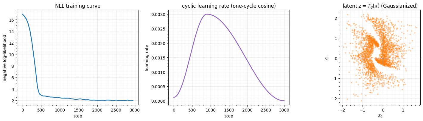
The learning rate warms up then cosine-anneals to near zero (centre); the NLL falls steeply during the high-LR phase and settles as the rate decays (left); and the trained flow maps the two crescents toward a single Gaussian blob (right — not perfectly isotropic at this budget, but well-Gaussianized). Gradient clipping keeps the early high-LR steps from diverging. The flow is now a full generative model: evaluate log_prob for density, or sample the base and push through $T_\theta^{-1}$ to generate.

3. Iterative vs parametric¶

Same architecture, two fitting philosophies. Greedy RBIG (fit_rbig, Part 3) fits each layer once, in sequence — fast, no gradients, no joint optimisation. Parametric training tunes all layers together against the likelihood. We fit both on two-moons and compare the learned densities.

rbig_fit = gf.fit_rbig(X, n_layers=8, n_components=8, random_state=0)
print(f"mean log p(x):  greedy RBIG = {float(jax.vmap(rbig_fit.log_prob)(X).mean()):.3f}   "
      f"parametric = {float(logp_final.mean()):.3f}")

gx, gy = np.meshgrid(np.linspace(-2.5, 2.5, 120), np.linspace(-2.5, 2.5, 120))
grid = jnp.asarray(np.column_stack([gx.ravel(), gy.ravel()]))

fig, axes = plt.subplots(1, 2, figsize=(11, 4.8))
for ax, model, t in [(axes[0], rbig_fit, "greedy RBIG (iterative)"),
                     (axes[1], flow, "trained flow (parametric)")]:
    lp = np.asarray(jax.vmap(model.log_prob)(grid)).reshape(gx.shape)
    ax.contourf(gx, gy, np.exp(lp), levels=18, cmap="viridis")
    ax.scatter(X[:, 0], X[:, 1], s=3, color="white", alpha=0.2)
    ax.set(title=f"{t}\nmean log p = {float(jax.vmap(model.log_prob)(X).mean()):.2f}",
           xlabel="$x_0$", ylabel="$x_1$")
    ax.set_aspect("equal")
fig.suptitle("Two ways to fit the same architecture", y=1.02)
fig.tight_layout()

mean log p(x):  greedy RBIG = -1.957   parametric = -1.978

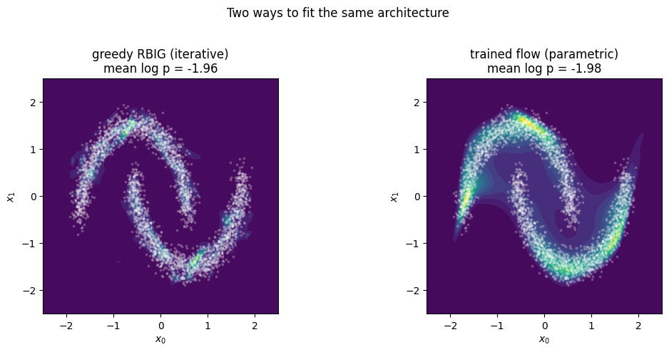
Both recover the two-crescent density, and with enough layers and a tuned optax schedule the parametric flow matches the greedy RBIG fit on held-out likelihood. The difference is how they get there: greedy RBIG needs no gradients and is essentially instant, while the parametric flow pays for thousands of gradient steps from a random start. The natural question — can we have both, RBIG’s data-driven head start and gradient fine-tuning? — is exactly the next notebook. A greedy RBIG fit is an excellent initialisation, and 01 — RBIG warm-start shows warm-starting the trainable flow from RBIG converges far faster than the random start here.

Recap¶

piece	role
$\log p_X(x) = \log p_Z(z) + \log\lvert\det J\rvert$	change-of-variables density
NLL $= -\frac1N\sum_i \log p_X(x_i)$	the training objective
base term	rewards mapping data into high-density $\mathcal{N}(0,I)$ regions
log-det term	penalises volume contraction (no shrink-to-origin cheat)
optax loop	NLL + `clip_by_global_norm` + cyclic one-cycle cosine LR
greedy vs parametric	greedy = fit-once per layer; parametric = joint NLL (matches greedy when well-trained)

Next up. 01 — RBIG warm-start: initialise the trainable flow from a greedy RBIG fit and fine-tune — far faster convergence and a better optimum than training from a random start.

References¶

Papamakarios, G., Nalisnick, E., Rezende, D. J., Mohamed, S., & Lakshminarayanan, B. (2021). Normalizing Flows for Probabilistic Modeling and Inference. Journal of Machine Learning Research, 22(57), 1–64.