RBIG rotation-choice studies - Research Notebook

02 — Rotation-choice studies¶

Every RBIG layer ends in a rotation (Part 2). Notebook 00 used PCA throughout, but the rotation is a real design choice — and a consequential one. It does not change where RBIG converges (any generic rotation reaches $\mathcal{N}(0,I)$ , the Laparra et al. guarantee Laparra et al. (2011)) but it sets how fast: a rotation that lands the data on informative axes lets the next marginal pass remove more dependence. We measure “fast” with the convergence yardstick of notebook 01 — the total correlation per layer — and compare the four rotations rbig provides.

What you will see

PCA, ICA, Picard drive the total correlation to zero in one layer on correlated data; a random rotation takes many.
Random still converges — the RBIG guarantee — just slowly; any generic rotation works, which is why random is a valid fit-free default.
Picard Ablin et al. (2018) as a fast, scalable ICA solver — the practical choice when you want ICA-quality rotations in higher dimensions.

import warnings

warnings.filterwarnings("ignore")

import matplotlib.pyplot as plt
import numpy as np

import rbig
from _style import style_ax

rng = np.random.default_rng(0)

# Correlated, near-Gaussian 4-D data: total correlation is reliably estimated here
# (notebook 01), positive, and large enough that the rotation choice clearly matters.
n = 3000
zsrc = rng.standard_normal((n, 4))
mix = np.array([[1, .8, .6, .4], [0, 1, .7, .5], [0, 0, 1, .6], [0, 0, 0, 1]], float)
X = zsrc @ mix.T
X = (X - X.mean(0)) / X.std(0)
print(f"initial total correlation = {float(rbig.total_correlation(X)):.3f} nats")

initial total correlation = 0.820 nats

1. Rotation choice sets the convergence speed¶

We run a short RBIG loop with each rotation and record the total correlation after every layer (the lower, the more independent — convergence). rbig provides PCARotation, ICARotation, RandomRotation, and PicardRotation; we drop each into the same marginal → rotate loop.

def tc_per_layer(rotation, n_layers=12, seed=0):
    """Total correlation after each RBIG layer, for a given rotation."""
    A = X.copy()
    tc = [float(rbig.total_correlation(A))]
    for k in range(n_layers):
        A = rbig.MarginalGaussianize().fit(A).transform(A)
        rot = {
            "PCA": rbig.PCARotation(whiten=False),
            "ICA": rbig.ICARotation(random_state=seed),
            "random": rbig.RandomRotation(random_state=seed + k),
            "Picard": rbig.PicardRotation(random_state=seed),
        }[rotation]
        A = rot.fit(A).transform(A)
        tc.append(float(rbig.total_correlation(A)))
    return np.abs(np.array(tc))

curves = {r: tc_per_layer(r) for r in ["PCA", "ICA", "Picard", "random"]}
print("layers to drive |TC| < 0.02:")
for r, v in curves.items():
    hit = next((i for i, x in enumerate(v) if x < 0.02), None)
    print(f"  {r:7s}: {hit if hit is not None else '>12'}")

fig, ax = plt.subplots(figsize=(7.8, 4.5))
colors = {"PCA": "tab:green", "ICA": "tab:blue", "Picard": "tab:purple", "random": "tab:red"}
for r, v in curves.items():
    ax.plot(v, "o-", color=colors[r], lw=2, ms=4, label=r)
ax.axhline(0.02, color="k", lw=1, ls="--", label="|TC| = 0.02 (converged)")
ax.set(title="Rotation choice sets RBIG convergence speed",
       xlabel="layer $k$", ylabel="total correlation $|T(x)|$ (nats)")
ax.legend(fontsize=9); style_ax(ax)
fig.tight_layout()

layers to drive |TC| < 0.02:
  PCA    : 1
  ICA    : 1
  Picard : 1
  random : >12

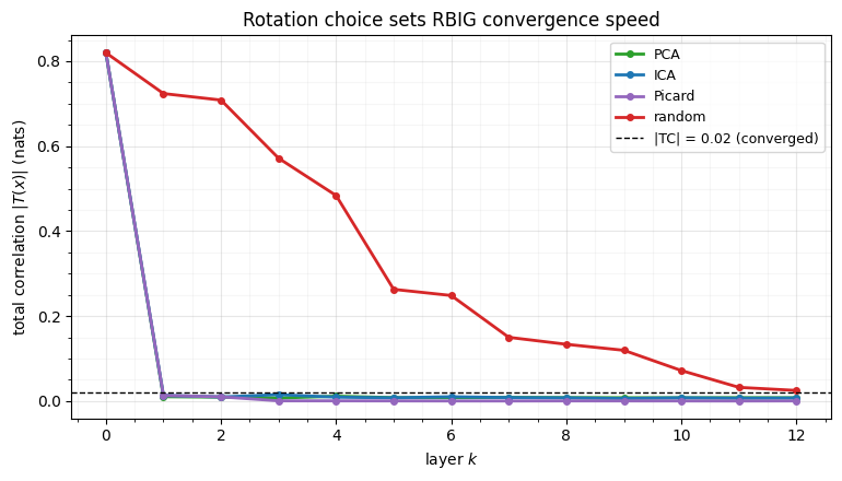
Data-driven rotations win. PCA, ICA, and Picard collapse the total correlation in a single layer — they each find axes aligned with the data’s structure, so the next marginal pass removes essentially all the dependence at once. The random rotation, blind to that structure, chips away slowly. Same destination, very different speed.

2. Random still converges — the RBIG guarantee¶

The slow red curve is not a failure. The theoretical heart of RBIG is that any generic (e.g. Haar-random) rotation drives the distribution to $\mathcal{N}(0,I)$ : each marginal pass can only reduce the total correlation, and a random rotation keeps re-exposing reducible structure. It just needs more layers. We extend it to confirm it gets there.

rand_long = tc_per_layer("random", n_layers=20)
reached = next((i for i, x in enumerate(rand_long) if x < 0.02), None)
print(f"random rotation reaches |TC| < 0.02 at layer {reached} "
      f"(vs 1 for PCA/ICA/Picard)")

# Geometry: covariance after ONE layer — PCA decorrelates, random does not.
def one_layer(rotation, seed=0):
    A = rbig.MarginalGaussianize().fit(X).transform(X)
    rot = (rbig.PCARotation(whiten=False) if rotation == "PCA"
           else rbig.RandomRotation(random_state=seed))
    return rot.fit(A).transform(A)

fig, axes = plt.subplots(1, 3, figsize=(13, 3.8))
for ax, (M, t) in zip(
    axes,
    [(np.cov(X.T), "input"),
     (np.cov(one_layer("PCA").T), "after 1 layer — PCA"),
     (np.cov(one_layer("random").T), "after 1 layer — random")],
):
    im = ax.imshow(np.abs(M), cmap="viridis", vmin=0, vmax=1)
    ax.set(title=t, xticks=range(4), yticks=range(4))
    fig.colorbar(im, ax=ax, fraction=0.046)
fig.suptitle("|covariance|: PCA decorrelates in one layer; random leaves structure", y=1.03)
fig.tight_layout()

random rotation reaches |TC| < 0.02 at layer 14 (vs 1 for PCA/ICA/Picard)

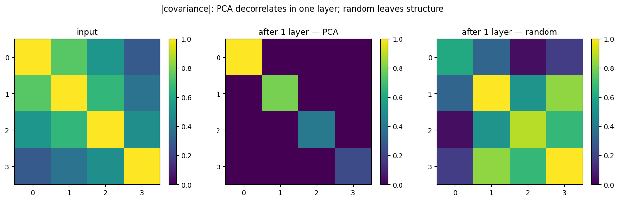
After a single layer PCA’s output covariance is diagonal (off-diagonals gone), while the random rotation’s still carries large off-diagonal dependence for the next pass to handle. So random is a perfectly valid, fit-free default — robust and assumption-light — you simply pay for it in depth.

3. Picard — a fast, scalable ICA for RBIG¶

PCA only removes linear correlation; ICA goes further, rotating onto maximally non-Gaussian (independent) axes Hyvärinen & Oja (2000), which is the better target when the data is a mix of non-Gaussian sources. Classic FastICA can be slow and finicky to converge in high dimensions. Picard Ablin et al. (2018) is a preconditioned quasi-Newton solver on the orthogonal manifold that optimises the same ICA objective far more robustly — the practical choice for ICA-based RBIG at scale. Here, on low-dimensional data, it matches ICA’s one-layer convergence.

import time

Xg = rbig.MarginalGaussianize().fit(X).transform(X)
for name, R in [("ICA   ", rbig.ICARotation(random_state=0)),
                ("Picard", rbig.PicardRotation(random_state=0))]:
    t0 = time.time()
    R.fit(Xg)
    dt = 1000 * (time.time() - t0)
    print(f"{name}: single-fit {dt:5.1f} ms, "
          f"|TC| after 1 layer = {abs(float(rbig.total_correlation(R.transform(Xg)))):.4f}")

print("\nICA and Picard both converge in one layer here; Picard's quasi-Newton "
      "solver is the one that keeps converging reliably as the dimension grows.")

ICA   : single-fit   7.0 ms, |TC| after 1 layer = 0.0132
Picard: single-fit   9.9 ms, |TC| after 1 layer = 0.0129

ICA and Picard both converge in one layer here; Picard's quasi-Newton solver is the one that keeps converging reliably as the dimension grows.

On this small problem ICA and Picard are neck-and-neck — both reach independence in one layer and take a few milliseconds. The reason to reach for Picard is dimension: its second-order updates converge in far fewer iterations than FastICA’s fixed-point steps as $d$ grows, so it is the rotation of choice when you want ICA-quality Gaussianization on high-dimensional data without the fitting cost blowing up.

Recap¶

rotation	finds	converges	cost	use when
PCA	variance axes (linear decorrelation)	~1 layer (Gaussian-ish data)	cheap	scales differ; near-Gaussian dependence
ICA	non-Gaussian / independent axes	~1 layer	moderate	mixed non-Gaussian sources
Picard	same ICA objective, quasi-Newton	~1 layer	moderate, scales well	ICA quality in high $d$
random	nothing (Haar)	many layers	free (no fit)	robust fit-free default

All reach $\mathcal{N}(0,I)$ ; the choice trades fitting cost against depth. The convergence signal of notebook 01 is the yardstick that makes the trade-off measurable.

Next up. One practical wrinkle remains: the marginal step relies on the empirical CDF, which is undefined past the data’s range and clips the tails to $\pm\infty$ under $\Phi^{-1}$ . 03 — Boundary issues & support extension handles tail behaviour, support extension, and dequantising discrete inputs — the last piece before Part 4 turns RBIG into a trainable parametric flow (where the RBIG warm-start lives).

References¶

Laparra, V., Camps-Valls, G., & Malo, J. (2011). Iterative Gaussianization: From ICA to Random Rotations. IEEE Transactions on Neural Networks, 22(4), 537–549. 10.1109/TNN.2011.2106511
Ablin, P., Cardoso, J.-F., & Gramfort, A. (2018). Faster Independent Component Analysis by Preconditioning with Hessian Approximations. IEEE Transactions on Signal Processing, 66(15), 4040–4049.
Hyvärinen, A., & Oja, E. (2000). Independent Component Analysis: Algorithms and Applications. Neural Networks, 13(4–5), 411–430.