Boundary issues & support extension

03 — Boundary issues & support extension¶

RBIG’s marginal step (Part 1 00) maps a coordinate through $z = \Phi^{-1}(\hat F(x))$ , where $\hat F$ is the empirical CDF. That works beautifully inside the data range — but the empirical CDF is flat at 0 below the smallest sample and at 1 above the largest, and $\Phi^{-1}(0) = -\infty$ , $\Phi^{-1}(1) = +\infty$ . Any point in the tails — a new test sample, or even a training point near the extremes — drives the transform toward $\pm\infty$ . This is the boundary problem, and it is exactly what produced the tail round-trip error we saw in notebook 00.

What you will see

The failure: an out-of-support point maps to nan/ $\pm\infty$ without bound correction.
The clip (bound_correct=True): finite, but tail information is lost, so the inverse degrades in the tails.
Support extension (pdf_extension): widen the CDF domain so the inverse is near-exact even in the tails (round-trip max error $1.3 \to 10^{-13}$ ).
Dequantisation: add uniform noise so discrete inputs stop collapsing into a staircase under the CDF.

import warnings

warnings.filterwarnings("ignore")

import matplotlib.pyplot as plt
import numpy as np
from scipy import stats

import rbig
from _style import style_ax

rng = np.random.default_rng(123)

# A skewed (Gamma) marginal: long right tail, so boundary effects are pronounced.
X = stats.gamma(a=4).rvs(size=(5000, 1), random_state=123)
print(f"training range: [{X.min():.2f}, {X.max():.2f}]")

training range: [0.17, 18.28]

1. The boundary problem¶

Take a point beyond the training range. Without bound correction the empirical CDF reads exactly 1 there and the probit diverges; with the default bound_correct=True, rbig clips the CDF to $[\varepsilon, 1-\varepsilon]$ so the output saturates at $\Phi^{-1}(1-\varepsilon) \approx 4.75$ instead of $+\infty$ .

X_oos = np.array([[X.max() + 5.0]])           # 5 units beyond the largest sample

z_raw = rbig.MarginalGaussianize(bound_correct=False).fit(X).transform(X_oos)[0, 0]
z_clip = rbig.MarginalGaussianize(bound_correct=True, eps=1e-6).fit(X).transform(X_oos)[0, 0]
print(f"out-of-support point x = {X_oos[0, 0]:.2f}")
print(f"  bound_correct=False : z = {z_raw}   (probit diverges)")
print(f"  bound_correct=True  : z = {z_clip:.3f}   (clipped to Phi^-1(1-eps), finite)")

out-of-support point x = 23.28
  bound_correct=False : z = nan   (probit diverges)
  bound_correct=True  : z = 4.753   (clipped to Phi^-1(1-eps), finite)

The clip is the right first line of defence — it keeps the pipeline numerically alive — and it is on by default. But clipping is lossy: every point past the $\varepsilon$ quantile is mapped to the same saturated value, so the map is no longer invertible there.

2. The cost of clipping: tail round-trip error¶

That saturation is precisely why the round-trip $x \to z \to x$ degraded in the tails in notebook 00. We confirm it: the median round-trip error is tiny, but the worst errors sit at the most extreme $|z|$ .

mg = rbig.MarginalGaussianize().fit(X)        # default: bound_correct=True
z = mg.transform(X)
X_rt = mg.inverse_transform(z)
err = np.abs(X - X_rt).ravel()
worst = np.argsort(err)[-5:]
print(f"round-trip error: median = {np.median(err):.2e}, max = {err.max():.3f}")
print(f"|z| at the 5 worst points: {np.round(np.abs(z.ravel()[worst]), 2)}  (all in the tails)")

fig, ax = plt.subplots(figsize=(7.4, 4.3))
ax.scatter(np.abs(z.ravel()), np.maximum(err, 1e-12), s=6, alpha=0.3, color="tab:red")
ax.set(title="Round-trip error concentrates in the tails (clipping)",
       xlabel=r"$|z|$ (distance into the tail)", ylabel=r"$|x - T^{-1}(T(x))|$",
       yscale="log")
style_ax(ax)
fig.tight_layout()

round-trip error: median = 1.78e-04, max = 1.318
|z| at the 5 worst points: [2.83 2.76 3.29 3.43 3.72]  (all in the tails)

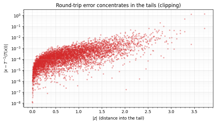
Inside $|z|\lesssim 2$ the round-trip is machine-accurate; past that it climbs by orders of magnitude as the clip throws away tail resolution. For Gaussianization of data this rarely matters, but for generation (inverting $z\sim\mathcal{N}(0,I)$ , which routinely draws $|z|>3$ ) it does — those are the smeared samples of notebook 00.

3. Support extension fixes the tails¶

The cure is to extend the support before building the CDF: pad the quantile domain beyond the observed range so the CDF has room to reach 0 and 1 smoothly instead of saturating at the data extremes. rbig.MarginalUniformize exposes this as pdf_extension (a percentage of the domain added on each side). Widening the support collapses the tail round-trip error by orders of magnitude.

for ext in [0.0, 5.0, 10.0]:
    mu = rbig.MarginalUniformize(bound_correct=True, eps=1e-6, pdf_extension=ext).fit(X)
    rt = np.abs(X - mu.inverse_transform(mu.transform(X))).max()
    print(f"pdf_extension = {ext:4.0f}%  ->  round-trip max error = {rt:.3e}")

# KDE marginals are the smooth alternative: their tails extend naturally.
kde = rbig.MarginalKDEGaussianize(eps=1e-6).fit(X)
print(f"\nMarginalKDEGaussianize: out-of-support z = {float(kde.transform(X_oos)[0, 0]):.3f} "
      f"(smooth KDE tail, finite)")

# Picture the extension: empirical CDF saturates; extended CDF reaches 0/1 past the data.
q = np.percentile(X.ravel(), np.linspace(0, 100, 200))
ref = np.linspace(0, 1, 200)
dom = q.max() - q.min()
q_ext = np.hstack([q.min() - 0.1 * dom, q, q.max() + 0.1 * dom])
ref_ext = np.interp(q_ext, q, ref)

fig, ax = plt.subplots(figsize=(7.4, 4.3))
ax.plot(q, ref, color="tab:red", lw=2, label="empirical CDF (saturates at data range)")
ax.plot(q_ext, ref_ext, "--", color="tab:green", lw=2, label="extended support (pdf_extension)")
ax.axvline(X.min(), color="k", lw=0.6, ls=":"); ax.axvline(X.max(), color="k", lw=0.6, ls=":")
ax.set(title="Support extension gives the CDF room to reach 0 and 1",
       xlabel="x", ylabel=r"$\hat F(x)$")
ax.legend(fontsize=8); style_ax(ax)
fig.tight_layout()

pdf_extension =    0%  ->  round-trip max error = 1.318e+00
pdf_extension =    5%  ->  round-trip max error = 1.066e-13
pdf_extension =   10%  ->  round-trip max error = 7.105e-14

MarginalKDEGaussianize: out-of-support z = 4.753 (smooth KDE tail, finite)

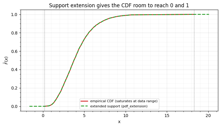
With a 10 % extension the round-trip is back to machine precision: the inverse no longer hits a saturated plateau. KDE marginals achieve a similar end differently — their density (and CDF) extend smoothly just past the training range, so points near the boundary get a graceful $z$ rather than a sharp plateau (a point far outside, like the +5 above, still saturates at the $\varepsilon$ clip). Either tool is what you want when you intend to sample from an RBIG model.

4. Dequantisation for discrete inputs¶

A different boundary pathology: discrete data. If $x$ takes only integer values, many samples tie, the empirical CDF is a staircase, and the probit maps every copy of a value to the same $z$ — the continuous Gaussianization collapses onto a few atoms. The standard fix is dequantisation: add uniform noise $u\sim\mathrm{Uniform}[0,1)$ to spread each integer over a unit interval before Gaussianizing (the surjection revisited in Part 8).

counts = rng.poisson(3, size=(5000, 1)).astype(float)        # discrete counts
z_disc = rbig.MarginalGaussianize().fit(counts).transform(counts)
deq = counts + rng.uniform(0, 1, counts.shape)               # dequantise
z_deq = rbig.MarginalGaussianize().fit(deq).transform(deq)

print(f"discrete:     {len(np.unique(counts))} input levels -> {len(np.unique(z_disc))} distinct z (staircase)")
print(f"dequantised:  -> {len(np.unique(z_deq))} distinct z, std = {z_deq.std():.3f}")

fig, axes = plt.subplots(1, 2, figsize=(11, 4.0), sharey=True)
axes[0].hist(z_disc.ravel(), bins=60, color="tab:red", alpha=0.8)
axes[0].set(title="discrete input → atoms in z", xlabel="z", ylabel="count")
axes[1].hist(z_deq.ravel(), bins=60, color="tab:green", alpha=0.8)
axes[1].set(title="dequantised (+U[0,1)) → smooth N(0,1)", xlabel="z")
for ax in axes:
    style_ax(ax)
fig.tight_layout()

discrete:     11 input levels -> 11 distinct z (staircase)
dequantised:  -> 5000 distinct z, std = 1.000

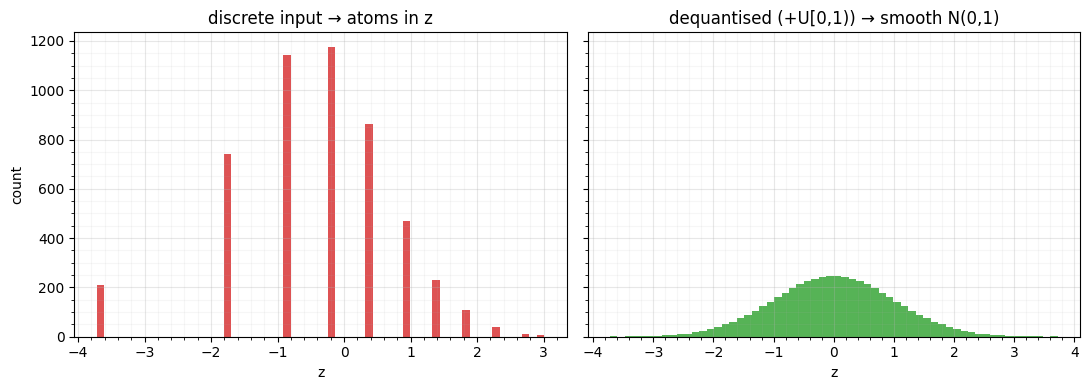
Without dequantisation the “Gaussianized” counts are a handful of spikes — useless for a continuous flow. Adding sub-integer noise turns the staircase into a smooth standard normal. (The noise is a stochastic surjection, with its own ELBO bookkeeping; Part 8 treats it properly.)

Recap¶

issue	symptom	fix
empirical-CDF tails	$\Phi^{-1}(0/1) = \pm\infty$	`bound_correct=True` clips to $[\varepsilon, 1-\varepsilon]$
clipping is lossy	tail round-trip error blows up	`pdf_extension` (extend support) or KDE marginals
discrete inputs	ties → staircase / atoms in $z$	dequantise: add $\mathrm{Uniform}[0,1)$ noise

These are the numerical guardrails that make RBIG dependable end to end — and the tail handling is what lets the generator of notebook 00 draw clean tail samples.

Part 3 → Part 4¶

That completes Iterative Gaussianization: the RBIG loop (00), its convergence and stopping rule (01), the rotation choices that set its speed (02), and the boundary care that makes it robust (03). RBIG is greedy and non-parametric — each layer fit once, never revisited. Part 4 — Parametric Gaussianization Flows makes the whole stack trainable: the same rotation + marginal blocks, but fit end-to-end by maximum likelihood — and that is where the RBIG warm-start (using a greedy RBIG fit to initialise a trainable flow) naturally belongs.