The canonical RBIG loop

00 — The canonical RBIG loop¶

We now have both halves of Gaussianization. Part 1 turns one coordinate into a standard normal; Part 2 mixes coordinates with a rotation so the next marginal pass has something to do. Rotation-Based Iterative Gaussianization Laparra et al. (2011) is the algorithm that stacks them:

x^{(k+1)} = Q_k\,\Psi_k\big(x^{(k)}\big),

((1))

where $\Psi_k$ is the per-coordinate marginal Gaussianization and $Q_k$ is an orthogonal rotation. Iterate, and the distribution flows to $\mathcal{N}(0,I)$ — a density destructor in the sense of Inouye & Ravikumar Inouye & Ravikumar (2018) (Part 0 04). Because every block is invertible, the whole stack is invertible: run it forward to evaluate density, backward to generate.

What you will see

One RBIG layer = marginal Gaussianization + rotation, built from rbig.
The morph: two-moons → $\mathcal{N}(0,I)$ , snapshot layer by layer.
Forward vs inverse: Gaussianize the data, then sample $\mathcal{N}(0,I)$ and run the layers in reverse to generate two-moons back.
Confirming against rbig.AnnealedRBIG and the smooth gauss_flows RBIG, whose exact log-det gives a trustworthy density.

import warnings

warnings.filterwarnings("ignore")

import jax
import jax.numpy as jnp
import jax.random as jr
import matplotlib.pyplot as plt
import numpy as np
from sklearn.datasets import make_moons

import gauss_flows as gf
import rbig
from _style import SCATTER_KW, style_ax

jax.config.update("jax_enable_x64", True)
rng = np.random.default_rng(0)

X, _ = make_moons(n_samples=4000, noise=0.07, random_state=0)
X = (X - X.mean(0)) / X.std(0)

1. One RBIG layer¶

A single layer does two things in sequence. First, marginal Gaussianization (Ψ): map each coordinate through $\Phi^{-1}(\hat F_i(x_i))$ so every axis becomes standard normal — but the joint stays dependent (Part 2 00 showed this alone stalls). Then a rotation ( $Q$ ): re-frame the coordinates so the next marginal pass sees fresh non-Gaussian structure. rbig.MarginalGaussianize and rbig.PCARotation are the two pieces.

mg = rbig.MarginalGaussianize().fit(X)
X_marg = mg.transform(X)
rot = rbig.PCARotation(whiten=False).fit(X_marg)
X_rot = rot.transform(X_marg)

fig, axes = plt.subplots(1, 3, figsize=(13.5, 4.2), sharex=True, sharey=True)
for ax, D, t in zip(axes, [X, X_marg, X_rot],
                    ["input (two-moons)", "after marginal $\\Psi$ (axes ~N(0,1))",
                     "after rotation $Q$ (re-framed)"]):
    ax.scatter(D[:, 0], D[:, 1], color="tab:blue", **SCATTER_KW)
    ax.set(title=t, xlabel="$x_0$")
    ax.axhline(0, color="k", lw=0.6); ax.axvline(0, color="k", lw=0.6)
    style_ax(ax)
axes[0].set_ylabel("$x_1$")
fig.suptitle("One RBIG layer = marginal Gaussianization, then rotation", y=1.02)
fig.tight_layout()
print(f"after marginal: per-axis std = {X_marg.std(0).round(3)}  (each ~1, but joint still moon-shaped)")

after marginal: per-axis std = [1. 1.]  (each ~1, but joint still moon-shaped)

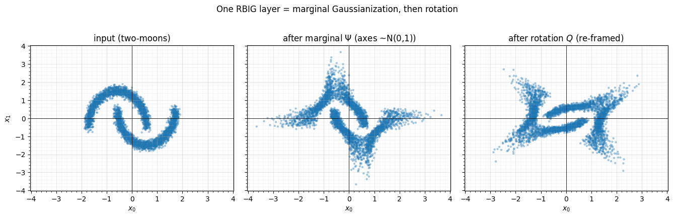
The marginal step makes each axis standard normal, but the cloud is still clearly two crescents — a separable map cannot remove that. The rotation mixes the axes; now the next layer’s marginal step has new structure to attack. Stacking this block is the whole algorithm.

2. The morph: two-moons → $\mathcal{N}(0,I)$ ¶

We build the loop from scratch — fit a layer, transform, repeat — keeping each intermediate state and the total correlation $\mathrm{TC}$ (Part 2’s dependence measure, 0 iff independent). Watch the crescents dissolve into an isotropic Gaussian blob.

def rbig_fit(X, n_layers, seed=0):
    """Fit an RBIG stack; return per-layer snapshots, TC trace, and the layers."""
    A = X.copy()
    snaps, tc, layers = [A.copy()], [float(rbig.total_correlation(A))], []
    for _ in range(n_layers):
        mg = rbig.MarginalGaussianize().fit(A); A = mg.transform(A)
        rot = rbig.PCARotation(whiten=False).fit(A); A = rot.transform(A)
        layers.append((mg, rot))
        snaps.append(A.copy()); tc.append(float(rbig.total_correlation(A)))
    return snaps, tc, layers

n_layers = 12
snaps, tc, layers = rbig_fit(X, n_layers)
Z = snaps[-1]
print(f"final latent: mean = {Z.mean():+.3f}, std = {Z.std():.3f}, "
      f"|TC| = {abs(tc[-1]):.4f}  (independent)")

# Our hand-rolled loop matches the maintained rbig.AnnealedRBIG implementation.
Z_ann = rbig.AnnealedRBIG(n_layers=50, rotation="pca", random_state=0).fit_transform(X)
print(f"rbig.AnnealedRBIG latent: mean = {Z_ann.mean():+.3f}, std = {Z_ann.std():.3f}, "
      f"|TC| = {abs(float(rbig.total_correlation(Z_ann))):.4f}")

show = [0, 1, 2, 4, 8, 12]
fig, axes = plt.subplots(1, len(show), figsize=(16, 3.0), sharex=True, sharey=True)
for ax, k in zip(axes, show):
    ax.scatter(snaps[k][:, 0], snaps[k][:, 1], color="tab:blue", **SCATTER_KW)
    ax.set(title=f"layer {k}", xlabel="$x_0$" if k else "input")
    ax.axhline(0, color="k", lw=0.5); ax.axvline(0, color="k", lw=0.5)
    ax.set_aspect("equal"); style_ax(ax)
fig.suptitle("RBIG morph: two-moons dissolves into N(0, I)", y=1.05)
fig.tight_layout()

final latent: mean = -0.000, std = 1.000, |TC| = 0.0002  (independent)

rbig.AnnealedRBIG latent: mean = -0.000, std = 1.000, |TC| = 0.0002

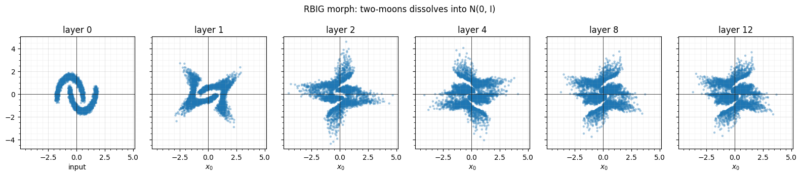
By a dozen layers the moons are an isotropic Gaussian and the total correlation has collapsed to (estimator) zero. Each layer chips away a little more non-Gaussianity — the formal monotone-decrease guarantee is the subject of notebook 01. Note the latent reaches $\mathcal{N}(0,I)$ in distribution; individual points are not preserved across the morph (it is a transport, not a labelling).

3. Forward for density, inverse for generation¶

Every block is invertible, so the stack runs both ways. Forward ( $x\to z$ ) is what we just did — Gaussianize the data. Inverse ( $z\to x$ ) runs the layers in reverse, each undoing its rotation then its marginal map; feed it $z\sim\mathcal{N}(0,I)$ and it generates new two-moons.

def rbig_inverse(Z, layers):
    A = Z.copy()
    for mg, rot in reversed(layers):
        A = rot.inverse_transform(A)
        A = mg.inverse_transform(A)
    return A

X_round = rbig_inverse(Z, layers)
err = np.abs(X - X_round).max(1)
print(f"round-trip error: median = {np.median(err):.2e}, max = {err.max():.2e} "
      f"(tails are worst — see notebook 04)")

round-trip error: median = 2.83e-03, max = 2.09e-01 (tails are worst — see notebook 04)

The round-trip is near machine precision in the bulk and degrades only in the tails (max $\sim0.2$ ), the boundary effect notebook 04 is devoted to. So the inverse mechanism is correct. Generation quality, though, depends on how smooth the marginal map is. Our from-scratch loop uses histogram marginals (Part 1 00): their inverse is piecewise-flat, so sampling $\mathcal{N}(0,I)$ and inverting yields a diffuse cloud — the moons are there but smeared. Swap in the smooth mixture-CDF marginals of gauss_flows’ RBIG (Part 1 01) and the same procedure generates crisp crescents. We sample both and compare.

Z_samp = rng.standard_normal((3000, 2))
X_gen_hist = rbig_inverse(Z_samp, layers)                    # histogram marginals (blocky)

res = gf.fit_rbig(jnp.asarray(X), n_layers=40, n_components=12, random_state=0)
X_gen_smooth = np.asarray(jax.vmap(res.sample)(jr.split(jr.key(0), 3000)))  # smooth mixture-CDF

fig, axes = plt.subplots(1, 3, figsize=(13.5, 4.6), sharex=True, sharey=True)
axes[0].scatter(X[:, 0], X[:, 1], color="tab:blue", **SCATTER_KW)
axes[0].set(title="data (two-moons)", xlabel="$x_0$", ylabel="$x_1$")
axes[1].scatter(X_gen_hist[:, 0], X_gen_hist[:, 1], color="tab:red", **SCATTER_KW)
axes[1].set(title="generated — histogram marginals (diffuse)", xlabel="$x_0$")
axes[2].scatter(X_gen_smooth[:, 0], X_gen_smooth[:, 1], color="tab:green", **SCATTER_KW)
axes[2].set(title="generated — smooth mixture-CDF (crisp)", xlabel="$x_0$")
for ax in axes:
    ax.set_aspect("equal"); ax.set(xlim=(-2.5, 2.5), ylim=(-2.5, 2.5)); style_ax(ax)
fig.suptitle(r"RBIG runs backwards to generate: $z\sim\mathcal{N}(0,I)\to T^{-1}(z)$", y=1.02)
fig.tight_layout()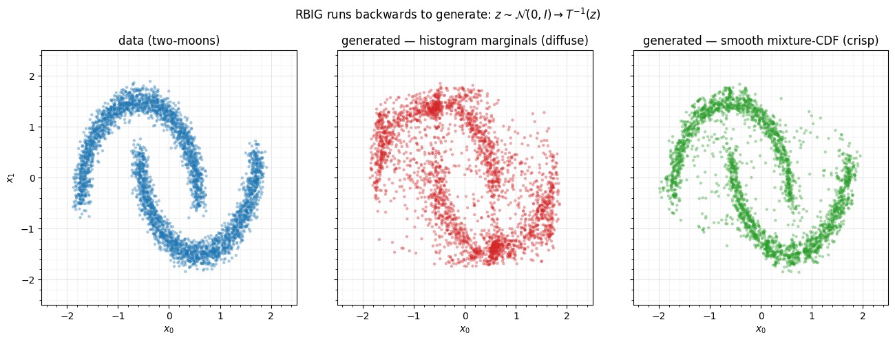

Same algorithm, same number of effective passes — the only difference is the marginal estimator. The histogram inverse scatters samples because its quantile function is a staircase; the smooth mixture-CDF inverse traces the manifold cleanly. The lesson generalises: for generation, use a smooth marginal; histograms are fine for a quick Gaussianization but blocky to sample from. This is also why the next notebooks lean on gauss_flows whenever sample/density quality matters.

4. The density¶

The same smooth gauss_flows RBIG gives a trustworthy density: with mixture-CDF marginals and an exact autodiff log-det, $\log p(x)$ is well-defined (unlike the histogram version, whose pointwise Jacobian is rough). On $\mathcal{N}(0,I)$ data its mean log-density matches the analytic value to two decimals; on two-moons its density concentrates on the crescents the generator samples.

# Sanity-check the density on N(0, I): mean log p should be the analytic -2.838.
G = jnp.asarray(rng.standard_normal((4000, 2)))
res_G = gf.fit_rbig(G, n_layers=12, n_components=12, random_state=0)
print(f"gf.fit_rbig log p on N(0,I): mean = {float(jax.vmap(res_G.log_prob)(G).mean()):.3f} "
      f"(analytic -2.838)")

# Density of the two-moons RBIG -> contour over the data.
gx, gy = np.meshgrid(np.linspace(-2.5, 2.5, 140), np.linspace(-2.5, 2.5, 140))
grid = jnp.asarray(np.column_stack([gx.ravel(), gy.ravel()]))
logp = np.asarray(jax.vmap(res.log_prob)(grid)).reshape(gx.shape)

fig, ax = plt.subplots(figsize=(5.6, 5.0))
ax.contourf(gx, gy, np.exp(logp), levels=18, cmap="viridis")
ax.scatter(X[:, 0], X[:, 1], s=4, color="white", alpha=0.25)
ax.set(title="gauss_flows RBIG density $p(x)$ (exact log-det)",
       xlabel="$x_0$", ylabel="$x_1$")
ax.set_aspect("equal")
fig.tight_layout()

gf.fit_rbig log p on N(0,I): mean = -2.849 (analytic -2.838)

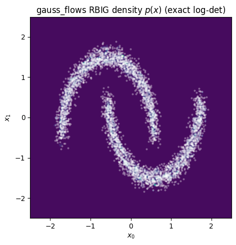
The learned density concentrates on the two crescents — the same object the generator samples from. Two takeaways for the rest of Part 3: rbig gives the canonical iterative algorithm and the information-theoretic measures (used next for convergence), while gauss_flows gives the smooth differentiable version whose exact log-det we trust for likelihoods and which Part 4 (parametric Gaussianization flows) fine-tunes end-to-end.

Recap¶

piece	role
marginal Ψ (Part 1)	makes each axis $\mathcal{N}(0,1)$ ; alone it stalls
rotation $Q$ (Part 2)	mixes axes so the next marginal pass progresses
stack $x^{(k+1)}=Q_k\Psi_k(x^{(k)})$	drives the joint to $\mathcal{N}(0,I)$ — a density destructor
forward $x\to z$	density / Gaussianization
inverse $z\to x$	generation (sample $\mathcal{N}(0,I)$ , invert)

Next up. We morphed for a fixed 12 layers. How many do we actually need, and how do we know we are done? 01 — Convergence & stopping shows that each layer provably reduces a non-Gaussianity measure (negentropy / total correlation), turning that into a principled stopping criterion.

References¶

Laparra, V., Camps-Valls, G., & Malo, J. (2011). Iterative Gaussianization: From ICA to Random Rotations. IEEE Transactions on Neural Networks, 22(4), 537–549. 10.1109/TNN.2011.2106511
Inouye, D. I., & Ravikumar, P. (2018). Deep Density Destructors. International Conference on Machine Learning (ICML).