Composable Models: Terms → Operators → Cycles

somax models plug into the pipekit ecosystem along three seams that build on each other. This tutorial walks the whole path end to end:

Terms — a model’s right-hand side as a sum of composable physics kernels, with per-term explicit/implicit tags for IMEX integration.
Operators — wrapping a built model as a pipekit.Operator: a one-step pipeline stage that satisfies pipekit_cycle.ForwardModel and (for flat-config models) round-trips through pipekit.serial.
Cycles — driving the stepping loop with pipekit_cycle.Cycle, threading state and collecting a trajectory.

The Operator/Cycle parts use pipekit, which is a base somax dependency (somax’s core still never imports it — conformance is structural). somax’s core never imports pipekit — models satisfy the protocols structurally.

from __future__ import annotations

import jax.numpy as jnp
import matplotlib.pyplot as plt
from pipekit import dumps, loads
from pipekit_cycle import Cycle, ForwardModel

from somax._src.models.swm.linear_2d import LinearSW2DState
from somax._src.models.swm.linear_swm_terms import LinearSWM2DTermModel
from somax.operators import Burgers2DOp, SomaxModelOp
from somax.solvers import imex_solver, imex_stepsize_controller

1. A model as a sum of term-kernels¶

The linear shallow water right-hand side decomposes into four distinct physics kernels — a gravity-wave (pressure) term, Coriolis, lateral diffusion, and bottom drag — that compose with +:

\texttt{rhs} = \underbrace{\texttt{gravity\_wave}}_{\text{fast, stiff}} + \texttt{coriolis} + \nu \cdot \underbrace{\texttt{diffusion}}_{\text{stiff}} + (-\kappa) \cdot \texttt{drag}

(1)

The differentiable parameters ( $\nu$ , $\kappa$ ) enter as Scaled coefficients (JAX leaves), so a loss can be differentiated straight through them.

model = LinearSWM2DTermModel.create(
    nx=64,
    ny=64,
    Lx=2_000e3,
    Ly=2_000e3,
    f0=1e-4,
    beta=2e-11,
    H0=100.0,
    lateral_viscosity=200.0,
    bottom_drag=1e-7,
)

# The assembled right-hand side is a Sum of four term-kernels:
for term in model.terms.terms:
    print(type(term).__name__, "->", repr(term))

print("\nviscosity nu read back from the tree:", float(model.nu))
print("bottom drag kappa read back from the tree:", float(model.kappa))

LinearSWMGravityWave -> LinearSWMGravityWave(
  diff=Difference2D(
    grid=CartesianGrid2D(
      Nx=66, Ny=66, Lx=2000000.0, Ly=2000000.0, dx=31250.0, dy=31250.0
    )
  ),
  g=9.81,
  H0=100.0
)
LinearSWMCoriolis -> LinearSWMCoriolis(
  coriolis=Coriolis2D(
    grid=CartesianGrid2D(
      Nx=66, Ny=66, Lx=2000000.0, Ly=2000000.0, dx=31250.0, dy=31250.0
    ),
    mask=None,
    interp=Interpolation2D(
      grid=CartesianGrid2D(
        Nx=66, Ny=66, Lx=2000000.0, Ly=2000000.0, dx=31250.0, dy=31250.0
      )
    )
  ),
  f_field=weak_f32[66,66]
)
Scaled -> Scaled(
  term=LinearSWMDiffusion(
    diff=Difference2D(
      grid=CartesianGrid2D(
        Nx=66, Ny=66, Lx=2000000.0, Ly=2000000.0, dx=31250.0, dy=31250.0
      )
    )
  ),
  coeff=weak_f32[]
)
Scaled -> Scaled(term=LinearSWMDrag(), coeff=weak_f32[])

viscosity nu read back from the tree: 200.0
bottom drag kappa read back from the tree: 1.0000000116860974e-07

2. IMEX — tag stiff terms implicit¶

Because each kernel carries an integration kind, a stiff term can be routed to the implicit stage of a splitting (IMEX) solver. With the default (all explicit) the whole RHS lowers to a single diffrax.ODETerm; with imex=True the diffusion term is tagged implicit and the RHS lowers to a diffrax.MultiTerm that an IMEX solver (e.g. KenCarp3) integrates with the stiff Laplacian handled implicitly.

explicit_model = LinearSWM2DTermModel.create(nx=32, ny=32, lateral_viscosity=200.0)
imex_model = LinearSWM2DTermModel.create(
    nx=32, ny=32, lateral_viscosity=200.0, imex=True
)

print("explicit build_terms():", type(explicit_model.build_terms()).__name__)
print("imex     build_terms():", type(imex_model.build_terms()).__name__)

explicit build_terms(): ODETerm
imex     build_terms(): MultiTerm

Integrating an IMEX model — use `somax.solvers.imex_solver`¶

An IMEX model needs an IMEX solver (KenCarp3, …) and an adaptive step-size controller — a fixed step with an implicit solver requires explicit tolerances. Just as important: the implicit stage must be solved matrix-free. diffrax.KenCarp3()'s default Newton root-finder materialises a dense N x N Jacobian (N = nx*ny), which is ~17 GB at 256 x 256 and OOMs (#55).

somax.solvers.imex_solver() returns a KenCarp3 whose implicit stage uses a Krylov (GMRES) Newton solve — O(N) memory, roughly flat runtime in resolution — and imex_stepsize_controller() is the matching adaptive controller. This is the recommended way to run any imex=True model.

imex_grid = imex_model.grid
gx = jnp.arange(imex_grid.Nx) * imex_grid.dx
gy = jnp.arange(imex_grid.Ny) * imex_grid.dy
gX, gY = jnp.meshgrid(gx, gy)
h_bump = jnp.exp(
    -0.5
    * (
        ((gX - gx[imex_grid.Nx // 2]) / (5 * imex_grid.dx)) ** 2
        + ((gY - gy[imex_grid.Ny // 2]) / (5 * imex_grid.dy)) ** 2
    )
)
imex_state0 = LinearSW2DState(
    h=h_bump, u=jnp.zeros_like(h_bump), v=jnp.zeros_like(h_bump)
)
imex_sol = imex_model.integrate(
    imex_state0,
    t0=0.0,
    t1=300.0,
    dt=30.0,
    solver=imex_solver(),
    stepsize_controller=imex_stepsize_controller(),
)
print("IMEX solve finite:", bool(jnp.all(jnp.isfinite(imex_sol.ys.h))))

IMEX solve finite: True

3. Wrap a built model as a pipekit Operator¶

SomaxModelOp turns any built somax model into a pipekit.Operator: a one-step stage (op(state) -> next_state) that also satisfies the pipekit_cycle.ForwardModel protocol (step / dt / state_signature).

op = SomaxModelOp(model, dt=90.0)
print("isinstance(op, ForwardModel):", isinstance(op, ForwardModel))
print("wrapped model:", type(op.model).__name__)

isinstance(op, ForwardModel): True
wrapped model: LinearSWM2DTermModel

4. Flat-config models round-trip through `pipekit.serial`¶

A built model is an eqx.Module (grids, operators, term trees) — not JSON primitives — so the general wrapper above is not serializable. Models whose construction is a flat primitive recipe expose a dedicated Operator (e.g. Burgers2DOp) whose config is all primitives, so dumps/loads round-trips the build recipe faithfully.

burgers = Burgers2DOp(nx=32, ny=32, nu=0.05, dt=1e-3, imex=False)
blob = dumps(burgers)
print("serialized config:", blob)

restored = loads(blob)
print("round-trip matches:", restored.get_config() == burgers.get_config())

serialized config: {"class": "Burgers2DOp", "config": {"Lx": 2.0, "Ly": 2.0, "dt": 0.001, "imex": false, "method": "upwind1", "nu": 0.05, "nx": 32, "ny": 32}, "module": "somax._src.operators"}
round-trip matches: True

5. Drive the model with `pipekit_cycle.Cycle`¶

Cycle applies the step operator n_steps times, threading state and (with save_history=True) collecting the trajectory. We seed a Gaussian height bump and watch gravity waves radiate outward under rotation — a geostrophic-adjustment problem. The gravity-wave term from step 1 is exactly what drives this.

grid = model.grid
x = jnp.arange(grid.Nx) * grid.dx
y = jnp.arange(grid.Ny) * grid.dy
X, Y = jnp.meshgrid(x, y)
cx, cy = grid.Nx * grid.dx / 2, grid.Ny * grid.dy / 2
sigma = grid.Nx * grid.dx / 12
h0 = jnp.exp(-0.5 * (((X - cx) / sigma) ** 2 + ((Y - cy) / sigma) ** 2))
state0 = LinearSW2DState(h=h0, u=jnp.zeros_like(h0), v=jnp.zeros_like(h0))

cycle = Cycle(step_op=op, n_steps=120, save_history=True, history_stride=20)
final_state, _ = cycle(state0, None)
print("steps recorded in history:", len(cycle.history))

steps recorded in history: 6

# Plot the initial bump and a few snapshots from the cycle history.
snapshots = [(0, state0)] + [
    (((i + 1) * cycle.history_stride), carrier)
    for i, (carrier, _state) in enumerate(cycle.history[:3])
]
fig, axes = plt.subplots(1, len(snapshots), figsize=(4 * len(snapshots), 3.6))
vmax = float(jnp.max(jnp.abs(h0)))
for ax, (step, st) in zip(axes, snapshots, strict=True):
    im = ax.pcolormesh(
        X / 1e3, Y / 1e3, st.h, cmap="RdBu_r", vmin=-vmax, vmax=vmax, shading="auto"
    )
    ax.set_title(f"step {step}  (t = {step * op.dt / 3600:.1f} h)")
    ax.set_xlabel("x [km]")
    ax.set_aspect("equal")
axes[0].set_ylabel("y [km]")
fig.colorbar(im, ax=axes, shrink=0.8, label="height h [m]")
plt.show()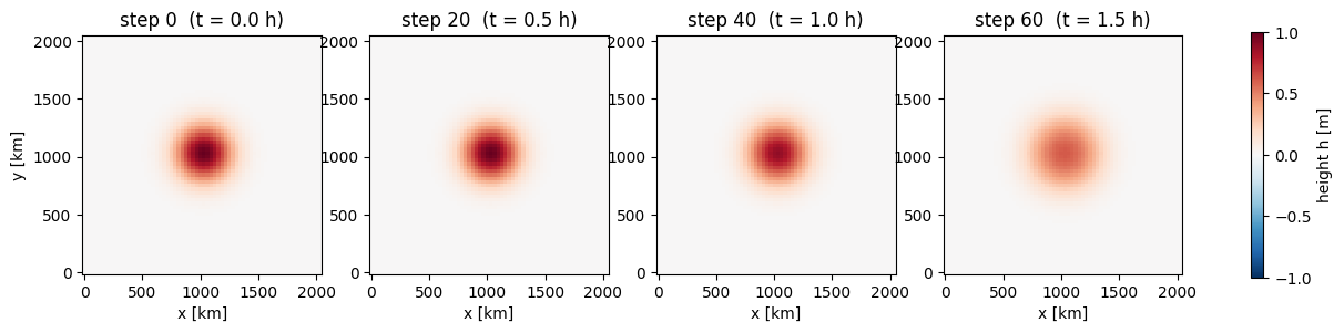

6. The `scenario x model` registry, end to end¶

SomaxModelOp.from_registry builds any compatible scenario x model pair through the dispatcher and hands back (op, state0) ready for Cycle. This is the full “what we simulate (scenario) x how we simulate it (model)” composition, wrapped as a pipekit Operator.

reg_op, reg_state0 = SomaxModelOp.from_registry(
    "double_gyre",
    "linear_swm",
    dt=60.0,
    scenario_params={"grid": {"nx": 16, "ny": 16}},
    model_params={"params": {"lateral_viscosity": 100.0, "bottom_drag": 1e-6}},
)
reg_final, _ = Cycle(step_op=reg_op, n_steps=10)(reg_state0, None)
print("built:", type(reg_op.model).__name__)
print("forward-integrated 10 steps; finite:", bool(jnp.all(jnp.isfinite(reg_final.h))))

# Operators compose like any pipekit stage — ``op | op`` is two steps.
two_steps = (reg_op | reg_op)(reg_state0)
print("op | op == two steps:", bool(jnp.all(jnp.isfinite(two_steps.h))))

built: LinearShallowWater2D
forward-integrated 10 steps; finite: True

op | op == two steps: True

Recap¶

Terms make a model’s RHS a transparent sum of physics kernels, with IMEX tags (gravity_wave + coriolis + nu*diffusion - kappa*drag).
Operators (SomaxModelOp / Burgers2DOp) expose a model as a pipekit stage + ForwardModel; flat-recipe models also serial round-trip.
Cycles drive the stepping loop and collect trajectories.

The same three seams power the somax-sim runner (which drives its chunked integration with Cycle) and let somax models plug into data-assimilation libraries (vardax, filterax) by satisfying ForwardModel structurally.

1. A model as a sum of term-kernels¶

2. IMEX — tag stiff terms implicit¶

Integrating an IMEX model — use somax.solvers.imex_solver¶

3. Wrap a built model as a pipekit Operator¶

4. Flat-config models round-trip through pipekit.serial¶

5. Drive the model with pipekit_cycle.Cycle¶

6. The scenario x model registry, end to end¶

Recap¶

Integrating an IMEX model — use `somax.solvers.imex_solver`¶

4. Flat-config models round-trip through `pipekit.serial`¶

5. Drive the model with `pipekit_cycle.Cycle`¶

6. The `scenario x model` registry, end to end¶