Data Assimilation — Ensemble Kalman Filtering with filterax
Somax models are forward operators; on their own they only propagate a
state. Data assimilation (DA) corrects that state against noisy, sparse
observations of reality. This tutorial wires a somax
Lorenz '96 model into
filterax and runs an Ensemble
Transform Kalman Filter (ETKF) twin experiment.
What you’ll learn:
The
somax.daadapters that bridge a somax model to a filterax filterHow to set up a twin experiment (truth run + synthetic observations)
How the analysis tracks the truth far better than a free forecast
The somax.da bridge
filterax filters operate on flat state vectors of shape (N_x,),
vectorised over an ensemble (N_e, N_x). somax states are equinox
pytrees. Three small adapters span that gap:
somax.da object | Role |
|---|---|
SomaxDynamics | wrap model.step as a filterax.AbstractDynamics |
SubsampleObs | sparse observation operator H(x) = x[indices] |
state_to_vector | flatten a state pytree to a vector (+ inverse) |
make_ensemble | build a perturbed flat ensemble around a state |
Because the dynamics adapter only relies on model.step(state, dt, *, t0=...),
any somax model drops in unchanged.
from __future__ import annotations

import jax
import jax.numpy as jnp
import lineax as lx
import matplotlib.pyplot as plt
from filterax import ETKF

from somax.da import SomaxDynamics, SubsampleObs, make_ensemble, state_to_vector
from somax.models import L96State, Lorenz96
1. The truth run
We use a 40-variable Lorenz '96 system at (fully chaotic). The truth
is spun up onto the attractor, then integrated forward in fixed windows of
dt = 0.05. This trajectory is what the filter is trying to recover — in a
real problem it is unknown.
key = jax.random.PRNGKey(0)
K = 40  # state dimension
dt = 0.05  # assimilation-window length
n_windows = 40  # number of observation times
n_members = 40  # ensemble size N_e
obs_var = 0.5  # observation-error variance

model = Lorenz96.create(F=8.0)
step = jax.jit(lambda s: model.step(s, dt))

# Spin the truth onto the attractor.
truth = L96State(x=8.0 * jnp.ones(K).at[0].add(0.01))
for _ in range(300):
    truth = step(truth)
truth0 = truth
print("truth spun up:", truth0.x.shape)
truth spun up: (40,)
2. Synthetic observations
We observe every other grid point (a 50% sparse network) with additive
Gaussian noise of variance obs_var. The observation operator is the linear
SubsampleObs; its error covariance R is a diagonal lineax operator.
obs_idx = jnp.arange(0, K, 2)  # observe x[0], x[2], x[4], ...
obs_op = SubsampleObs(indices=obs_idx)
R = lx.DiagonalLinearOperator(obs_var * jnp.ones(obs_idx.size))

truths, observations = [], []
state = truth0
for w in range(1, n_windows + 1):
    state = step(state)
    vec, _ = state_to_vector(state)
    truths.append(vec)
    key, sub = jax.random.split(key)
    noise = jnp.sqrt(obs_var) * jax.random.normal(sub, (obs_idx.size,))
    observations.append((vec[obs_idx] + noise, w * dt))
truths = jnp.stack(truths)  # (T, N_x)
print(f"{len(observations)} observation windows, {obs_idx.size} obs / window")
40 observation windows, 20 obs / window
3. Run the ETKF
The ensemble is seeded by perturbing the (known) initial truth — a stand-in
for background uncertainty. ETKF.assimilate then loops
forecast → analysis over every window. The forecast step is
SomaxDynamics (i.e. the somax model) vectorised over the ensemble; the
analysis is filterax’s ETKF update.
key, sub = jax.random.split(key)
ensemble0 = make_ensemble(truth0, sub, size=n_members, std=1.0)

etkf = ETKF(dynamics=SomaxDynamics(model=model, template=truth0), obs_op=obs_op)
result = etkf.assimilate(ensemble0, observations, R, t0=0.0)

analysis_mean = result.analysis_history.mean(axis=1)  # (T, N_x)
forecast_mean = result.forecast_history.mean(axis=1)  # (T, N_x)

analysis_rmse = jnp.sqrt(jnp.mean((analysis_mean - truths) ** 2, axis=1))
forecast_rmse = jnp.sqrt(jnp.mean((forecast_mean - truths) ** 2, axis=1))
print(f"mean analysis RMSE: {analysis_rmse.mean():.3f}")
print(f"mean forecast RMSE: {forecast_rmse.mean():.3f}")
print(f"observation-noise floor (sqrt obs_var): {jnp.sqrt(obs_var):.3f}")
mean analysis RMSE: 0.315
mean forecast RMSE: 0.338
observation-noise floor (sqrt obs_var): 0.707
4. Does it work?
Two checks. (a) the per-window RMSE of the analysis sits below the forecast and well under the observation-noise floor — the filter extracts more signal than any single observation carries. (b) the analysis Hovmoller is visually indistinguishable from the truth.
times = jnp.arange(1, n_windows + 1) * dt

fig, ax = plt.subplots(figsize=(7, 4))
ax.plot(times, forecast_rmse, label="forecast (prior)", lw=2)
ax.plot(times, analysis_rmse, label="analysis (posterior)", lw=2)
ax.axhline(float(jnp.sqrt(obs_var)), ls="--", c="grey", label="obs-noise floor")
ax.set(xlabel="time", ylabel="RMSE vs truth", title="ETKF analysis vs forecast")
ax.legend()
fig.tight_layout()
plt.show()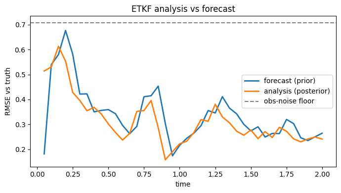
fig, axes = plt.subplots(1, 3, figsize=(12, 4), sharey=True)
kw = dict(aspect="auto", cmap="RdBu_r", vmin=-8, vmax=8, origin="lower")
axes[0].imshow(truths.T, **kw)
axes[0].set(title="truth", xlabel="window", ylabel="grid point $k$")
axes[1].imshow(analysis_mean.T, **kw)
axes[1].set(title="analysis mean", xlabel="window")
im = axes[2].imshow(
    (analysis_mean - truths).T,
    aspect="auto",
    cmap="RdBu_r",
    vmin=-2,
    vmax=2,
    origin="lower",
)
axes[2].set(title="analysis error", xlabel="window")
fig.colorbar(im, ax=axes, shrink=0.8, label="error")
plt.show()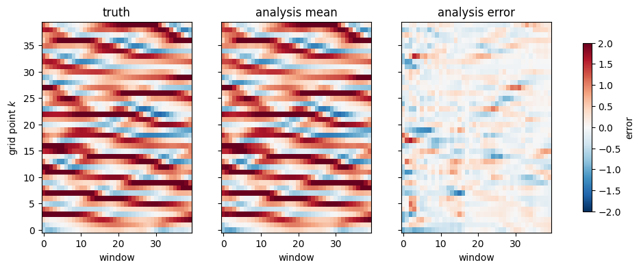
Summary
somax.daprovides the thin adapter layer (SomaxDynamics,SubsampleObs,state_to_vector,make_ensemble) that lets any somax model be driven by afilteraxensemble filter.In a Lorenz '96 twin experiment the ETKF analysis tracks the truth with RMSE below both the free forecast and the observation-noise floor, from sparse (50%) noisy observations.
The same pattern works for the shallow-water and QG models — swap the model and the
templatestate; the bridge is unchanged.
Variational assimilation (vardax 4DVar) with structured gaussx
background/observation covariances builds on the same somax.da surface.