Lorenz '63 — Your First somax Simulation - somax: Simple Ocean Models in JAX

The Lorenz '63 system is the canonical low-dimensional chaotic attractor. It is the simplest model in somax and a good starting point for understanding the API.

What you’ll learn:

How to create a model, state, and run a forward simulation
How the SomaxModel contract works (vector_field, integrate, diagnose)
How to differentiate through a simulation with jax.grad
How to run an ensemble with jax.vmap

Background¶

The system is defined by three coupled ODEs with parameters $\sigma$ (Prandtl number), $\rho$ (Rayleigh number), and $\beta$ (geometric factor):

\frac{dx}{dt} = \sigma(y - x), \qquad \frac{dy}{dt} = x(\rho - z) - y, \qquad \frac{dz}{dt} = xy - \beta z

(1)

At the standard parameters $(\sigma, \rho, \beta) = (10, 28, 8/3)$ the system exhibits deterministic chaos: nearby trajectories diverge exponentially, tracing the famous butterfly-shaped strange attractor.

from __future__ import annotations

import diffrax as dfx
import equinox as eqx
import jax
import jax.numpy as jnp
import jax.random as jrandom
import matplotlib.pyplot as plt

from somax.models import L63State, Lorenz63

1. Create the model¶

Lorenz63.create() builds a model with the standard parameter values. The model is an eqx.Module — an immutable pytree whose fields (including params) are visible to jax.grad and jax.jit.

model = Lorenz63.create(sigma=10.0, rho=28.0, beta=8.0 / 3.0)
print(model)

Lorenz63(params=L63Params(sigma=weak_f32[], rho=weak_f32[], beta=weak_f32[]))

2. Forward simulation¶

model.integrate() wraps diffrax.diffeqsolve with automatic boundary-condition enforcement. We save the trajectory at dense output times to visualize the attractor.

state0 = L63State(x=jnp.array(1.0), y=jnp.array(1.0), z=jnp.array(1.0))

t0, t1, dt = 0.0, 40.0, 0.01
ts = jnp.arange(t0, t1, dt)

sol = model.integrate(
    state0,
    t0=t0,
    t1=t1,
    dt=dt,
    saveat=dfx.SaveAt(ts=ts),
)

print(f"Trajectory shape: x={sol.ys.x.shape}, y={sol.ys.y.shape}, z={sol.ys.z.shape}")

Trajectory shape: x=(4000,), y=(4000,), z=(4000,)

3. Visualize the attractor¶

The classic 3D butterfly and the three time series.

colors = {
    "trajectory": "#2196F3",
    "start": "#4CAF50",
    "x": "#2196F3",
    "y": "#FF9800",
    "z": "#9C27B0",
}

fig = plt.figure(figsize=(14, 5))

# --- 3D attractor ---
ax3d = fig.add_subplot(121, projection="3d")
ax3d.plot(
    sol.ys.x,
    sol.ys.y,
    sol.ys.z,
    lw=0.4,
    alpha=0.8,
    color=colors["trajectory"],
)
ax3d.scatter(
    [sol.ys.x[0]],
    [sol.ys.y[0]],
    [sol.ys.z[0]],
    s=60,
    c=colors["start"],
    edgecolors="k",
    linewidths=0.5,
    zorder=5,
    label="IC",
)
ax3d.set_xlabel("x")
ax3d.set_ylabel("y")
ax3d.set_zlabel("z")
ax3d.set_title("Lorenz '63 attractor")
ax3d.legend(loc="upper left", fontsize=9)

# --- Time series ---
ax_ts = fig.add_subplot(122)
ax_ts.plot(ts, sol.ys.x, lw=0.8, color=colors["x"], label="x(t)")
ax_ts.plot(ts, sol.ys.y, lw=0.8, color=colors["y"], label="y(t)")
ax_ts.plot(ts, sol.ys.z, lw=0.8, color=colors["z"], label="z(t)")
ax_ts.set_xlabel("Time")
ax_ts.set_ylabel("State")
ax_ts.set_title("Time series")
ax_ts.legend(fontsize=9)
ax_ts.grid(True, alpha=0.3)

plt.tight_layout()
plt.show()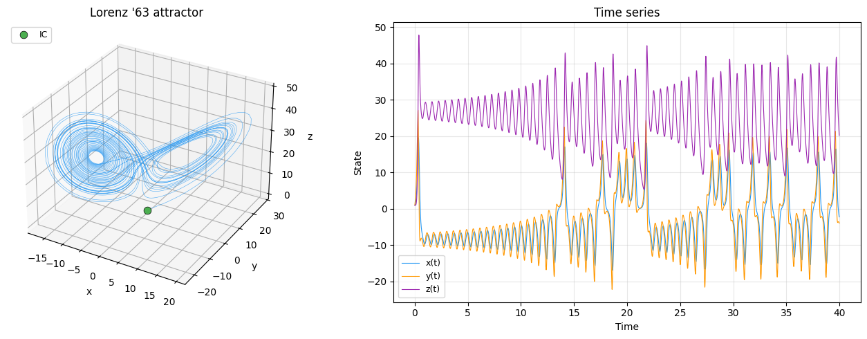

4. Diagnostics¶

model.diagnose() computes on-demand quantities from the state. For L63 it returns the kinetic energy $E = \tfrac{1}{2}(x^2 + y^2 + z^2)$ .

energy = jax.vmap(model.diagnose)(sol.ys).energy

fig, ax = plt.subplots(figsize=(10, 3))
ax.plot(ts, energy, lw=0.8, color="#F44336")
ax.set_xlabel("Time")
ax.set_ylabel("Energy")
ax.set_title("Kinetic energy along the trajectory")
ax.grid(True, alpha=0.3)
plt.tight_layout()
plt.show()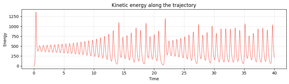

5. Adjoint methods for differentiation¶

Differentiating through an ODE solve requires an adjoint method that trades off memory, accuracy, and speed. diffrax provides three:

Adjoint	Memory	Gradients	Use case
`RecursiveCheckpointAdjoint`	$O(\sqrt{N})$	Exact	Default
`DirectAdjoint`	$O(N)$	Exact	Short windows
`BacksolveAdjoint`	$O(1)$	Approx	Long windows
`ImplicitAdjoint`	$O(1)$	Exact	Steady states

RecursiveCheckpointAdjoint (the default) uses Griewank--Walther optimal checkpointing: it re-computes forward steps from saved checkpoints during the backward pass, giving exact gradients with sub-linear memory.
DirectAdjoint stores the entire forward trajectory — exact but $O(N)$ memory. Also supports forward-mode AD.
BacksolveAdjoint solves the continuous adjoint ODE backwards in time with $O(1)$ memory. Gradients are approximate (optimize-then-discretize $\neq$ discretize-then-optimize).
ImplicitAdjoint differentiates through the implicit function theorem: if the solver finds a fixed point $u^*$ such that $g(u^*, \theta) = 0$ , the gradient is $du^*/d\theta = -(dg/du)^{-1}\, dg/d\theta$ . Memory is $O(1)$ and gradients are exact, but only applies to steady-state / fixed-point problems (not time-stepping).

5a. Gradient with respect to parameters¶

Use case: parameter estimation. Given observations, find the parameters $\theta = (\sigma, \rho, \beta)$ that minimize a loss.

We compute $\nabla_\theta \mathcal{L}$ where $\mathcal{L} = \sum_t \| \mathbf{u}(t) \|^2$ and the state $\mathbf{u}(t)$ depends on $\theta$ through the ODE:

\frac{\partial \mathcal{L}}{\partial \theta} = \int_0^T \lambda(t)^\top \frac{\partial f}{\partial \theta}\, dt

(2)

where $\lambda(t)$ is the adjoint state satisfying the backward ODE $\dot{\lambda} = -(\partial f / \partial u)^\top \lambda$ .

state0_grad = L63State(x=jnp.array(1.0), y=jnp.array(1.0), z=jnp.array(1.0))


@eqx.filter_grad
def grad_params(model):
    sol = model.integrate(state0_grad, t0=0.0, t1=1.0, dt=0.01)
    return jnp.sum(sol.ys.x**2 + sol.ys.y**2 + sol.ys.z**2)


grads_theta = grad_params(model)

print("--- Gradient w.r.t. parameters ---")
print(f"  dL/d(sigma) = {grads_theta.params.sigma:.4f}")
print(f"  dL/d(rho)   = {grads_theta.params.rho:.4f}")
print(f"  dL/d(beta)  = {grads_theta.params.beta:.4f}")

--- Gradient w.r.t. parameters ---
  dL/d(sigma) = -2.7039
  dL/d(rho)   = 15.1506
  dL/d(beta)  = 331.9404

5b. Gradient with respect to the initial state¶

Use case: state estimation / data assimilation. Given a model with known parameters, find the initial condition $\mathbf{u}_0$ that best fits observations (the 4D-Var problem).

We compute $\nabla_{\mathbf{u}_0} \mathcal{L}$ :

\frac{\partial \mathcal{L}}{\partial \mathbf{u}_0} = \lambda(0)

(3)

where $\lambda(t)$ is the same adjoint state, but now evaluated at $t = 0$ . This is the gradient that 4D-Var minimizes.

def loss_state(state0):
    sol = model.integrate(state0, t0=0.0, t1=1.0, dt=0.01)
    return jnp.sum(sol.ys.x**2 + sol.ys.y**2 + sol.ys.z**2)


grads_u0 = jax.grad(loss_state)(state0_grad)

print("--- Gradient w.r.t. initial state ---")
print(f"  dL/d(x0) = {grads_u0.x:.4f}")
print(f"  dL/d(y0) = {grads_u0.y:.4f}")
print(f"  dL/d(z0) = {grads_u0.z:.4f}")

--- Gradient w.r.t. initial state ---
  dL/d(x0) = -21.0361
  dL/d(y0) = -18.2364
  dL/d(z0) = 39.6907

5c. Joint gradient — parameters and state¶

Use case: bi-level optimization. Simultaneously estimate the initial state and model parameters (e.g. weak-constraint 4D-Var).

We compute $(\nabla_{\mathbf{u}_0} \mathcal{L}$ , $\nabla_\theta \mathcal{L})$ in a single backward pass using eqx.partition to separate the differentiable leaves.

def loss_joint(state0, model):
    sol = model.integrate(state0, t0=0.0, t1=1.0, dt=0.01)
    return jnp.sum(sol.ys.x**2 + sol.ys.y**2 + sol.ys.z**2)


grads_u0_joint, grads_model_joint = jax.grad(loss_joint, argnums=(0, 1))(
    state0_grad, model
)

print("--- Joint gradient ---")
print(f"  dL/d(x0)    = {grads_u0_joint.x:.4f}")
print(f"  dL/d(y0)    = {grads_u0_joint.y:.4f}")
print(f"  dL/d(z0)    = {grads_u0_joint.z:.4f}")
print(f"  dL/d(sigma) = {grads_model_joint.params.sigma:.4f}")
print(f"  dL/d(rho)   = {grads_model_joint.params.rho:.4f}")
print(f"  dL/d(beta)  = {grads_model_joint.params.beta:.4f}")

--- Joint gradient ---
  dL/d(x0)    = -21.0361
  dL/d(y0)    = -18.2364
  dL/d(z0)    = 39.6907
  dL/d(sigma) = -2.7039
  dL/d(rho)   = 15.1506
  dL/d(beta)  = 331.9404

5d. Comparing adjoint methods¶

We time RecursiveCheckpointAdjoint (default) vs DirectAdjoint on the same problem. BacksolveAdjoint requires passing the model as an explicit argument to diffeqsolve (not via closure), so it needs a different API pattern — see the diffrax docs for details.

import time


def timed_grad(adjoint, label):
    @eqx.filter_grad
    def fn(model):
        sol = model.integrate(state0_grad, t0=0.0, t1=1.0, dt=0.01, adjoint=adjoint)
        return jnp.sum(sol.ys.x**2 + sol.ys.y**2 + sol.ys.z**2)

    # Warm-up (JIT compilation)
    g = fn(model)
    jax.block_until_ready(g.params.sigma)
    # Timed run
    t_start = time.perf_counter()
    g = fn(model)
    jax.block_until_ready(g.params.sigma)
    elapsed = time.perf_counter() - t_start
    print(f"  {label:35s}  dL/d(sigma)={g.params.sigma:.4f}  ({elapsed:.4f}s)")


print("--- Adjoint method comparison ---")
timed_grad(dfx.RecursiveCheckpointAdjoint(), "RecursiveCheckpoint")
timed_grad(dfx.DirectAdjoint(), "Direct")

--- Adjoint method comparison ---

  RecursiveCheckpoint                  dL/d(sigma)=-2.7039  (5.1276s)

  Direct                               dL/d(sigma)=-2.7036  (3.1110s)

6. Ensemble simulation with `jax.vmap`¶

Chaotic systems are sensitive to initial conditions. We can explore this by running an ensemble of trajectories with small perturbations and watching them diverge.

n_ensemble = 50
key = jrandom.PRNGKey(42)
perturbations = 0.01 * jrandom.normal(key, shape=(n_ensemble, 3))

ensemble_states = L63State(
    x=1.0 + perturbations[:, 0],
    y=1.0 + perturbations[:, 1],
    z=1.0 + perturbations[:, 2],
)

ts_ens = jnp.arange(0.0, 30.0, 0.01)


def integrate_one(state0):
    return model.integrate(
        state0,
        t0=0.0,
        t1=30.0,
        dt=0.01,
        saveat=dfx.SaveAt(ts=ts_ens),
    )


ensemble_sol = eqx.filter_vmap(integrate_one)(ensemble_states)

fig, axes = plt.subplots(1, 3, figsize=(15, 4), sharey=False)

for ax, var, name, color in zip(
    axes,
    [ensemble_sol.ys.x, ensemble_sol.ys.y, ensemble_sol.ys.z],
    ["x(t)", "y(t)", "z(t)"],
    [colors["x"], colors["y"], colors["z"]],
    strict=True,
):
    for j in range(n_ensemble):
        ax.plot(ts_ens, var[j], lw=0.3, alpha=0.4, color=color)
    ax.set_xlabel("Time")
    ax.set_ylabel(name)
    ax.set_title(f"Ensemble — {name}")
    ax.grid(True, alpha=0.3)

plt.suptitle(
    f"Ensemble of {n_ensemble} trajectories (perturbation = 0.01)",
    fontsize=13,
)
plt.tight_layout()
plt.show()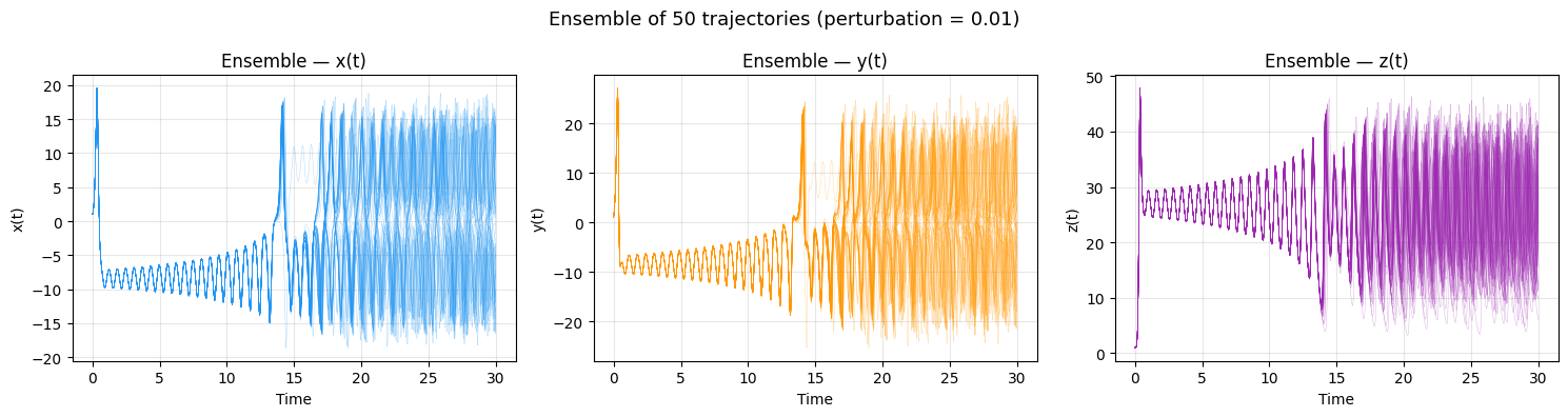

Summary¶

Concept	somax API
Create a model	`Lorenz63.create(sigma=10, rho=28, beta=8/3)`
Initial condition	`L63State(x=..., y=..., z=...)`
Forward simulation	`model.integrate(state0, t0, t1, dt, saveat=...)`
Diagnostics	`model.diagnose(state)`
Grad w.r.t. params	`eqx.filter_grad(loss)(model)`
Grad w.r.t. state	`jax.grad(loss)(state0)`
Joint grad	`jax.grad(loss, argnums=(0, 1))(state0, model)`
Ensemble	`eqx.filter_vmap(integrate_one)(batch_states)`

Next steps:

Try the Lorenz '96 tutorial for a higher-dimensional chaotic system
Explore the Shallow Water Model for your first PDE simulation

Lorenz '63 — Your First somax Simulation