Lorenz '96 — High-Dimensional Chaos - somax: Simple Ocean Models in JAX

The Lorenz '96 system is a periodic 1D lattice of $N$ coupled variables driven by a constant forcing $F$ . It is a workhorse model for testing data assimilation and ensemble forecasting methods.

What you’ll learn:

How to set up and run a high-dimensional chaotic ODE in somax
How the Hovmoller diagram reveals wave-like propagation
How forcing strength $F$ controls the transition to chaos
How to compute gradients and run ensembles at scale

Background¶

The system consists of $N$ variables $X_k$ on a periodic ring:

\frac{dX_k}{dt} = \underbrace{(X_{k+1} - X_{k-2})\, X_{k-1}}_{\text{advection}} - X_k + F \qquad k = 1, \ldots, N

(1)

with periodic boundary conditions $X_{k+N} = X_k$ .

The quadratic term mimics nonlinear advection (energy-conserving).
The linear damping $-X_k$ dissipates energy.
The constant forcing $F$ injects energy.

At $F = 8$ the system is fully chaotic with a doubling time of approximately 0.42 time units (about 2.1 days if one time unit equals 5 days).

from __future__ import annotations

import diffrax as dfx
import equinox as eqx
import jax
import jax.numpy as jnp
import jax.random as jrandom
import matplotlib.pyplot as plt

from somax.models import L96State, Lorenz96

1. Create the model¶

We use $N = 360$ variables for a smooth Hovmoller diagram. Lorenz’s original choice was $N = 40$ ; the higher resolution reveals finer-scale wave structure on the periodic ring.

N = 360
model = Lorenz96.create(F=8.0)
print(model)

Lorenz96(params=L96Params(F=weak_f32[]))

2. Forward simulation¶

The initial condition is a small perturbation of the $F$ -equilibrium state $X_k = F$ for all $k$ . This is an unstable fixed point of the system — the perturbation grows and the trajectory settles onto the chaotic attractor.

state0 = L96State.init_state(ndim=N, noise=0.01, F=8.0)

t0, t1, dt = 0.0, 20.0, 0.005
ts = jnp.arange(t0, t1, dt)

sol = model.integrate(
    state0,
    t0=t0,
    t1=t1,
    dt=dt,
    saveat=dfx.SaveAt(ts=ts),
)

print(f"Trajectory shape: {sol.ys.x.shape}")  # (T, N)

Trajectory shape: (4000, 360)

3. Hovmoller diagram¶

A Hovmoller plot shows the state as a function of position (x-axis) and time (y-axis). The tilted bands reveal wave-like structures propagating around the periodic ring.

fig, ax = plt.subplots(figsize=(10, 6))
im = ax.imshow(
    sol.ys.x,
    aspect="auto",
    origin="lower",
    cmap="RdBu_r",
    vmin=-10,
    vmax=15,
    extent=[0, N, float(ts[0]), float(ts[-1])],
    interpolation="bilinear",
)
ax.set_xlabel("Variable index $k$")
ax.set_ylabel("Time")
ax.set_title(f"Hovmoller diagram — Lorenz '96 ($N={N}$, $F=8$)")
plt.colorbar(im, ax=ax, label="$X_k$")
plt.tight_layout()
plt.show()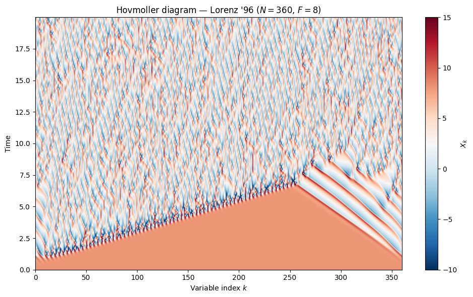

4. Time series and statistics¶

Individual variables look like noisy oscillations. The climatological mean is close to $F$ and the variance grows with forcing strength.

colors = ["#2196F3", "#FF9800", "#4CAF50", "#9C27B0", "#F44336"]

fig, axes = plt.subplots(2, 1, figsize=(12, 6), sharex=True)

# Top: a few selected variables
ax = axes[0]
for i, c in zip([0, 90, 180, 270], colors, strict=False):
    ax.plot(ts, sol.ys.x[:, i], lw=0.6, alpha=0.8, color=c, label=f"$X_{{{i}}}$")
ax.set_ylabel("$X_k$")
ax.set_title("Selected variables")
ax.legend(fontsize=9, ncol=4)
ax.grid(True, alpha=0.3)

# Bottom: spatial mean and std
spatial_mean = jnp.mean(sol.ys.x, axis=1)
spatial_std = jnp.std(sol.ys.x, axis=1)
ax = axes[1]
ax.plot(ts, spatial_mean, lw=1, color="#2196F3", label="Spatial mean")
ax.fill_between(
    ts,
    spatial_mean - spatial_std,
    spatial_mean + spatial_std,
    alpha=0.2,
    color="#2196F3",
    label=r"$\pm 1\sigma$",
)
ax.axhline(8.0, color="k", ls="--", lw=0.8, alpha=0.5, label="$F = 8$")
ax.set_xlabel("Time")
ax.set_ylabel("$X_k$")
ax.set_title("Spatial statistics")
ax.legend(fontsize=9)
ax.grid(True, alpha=0.3)

plt.tight_layout()
plt.show()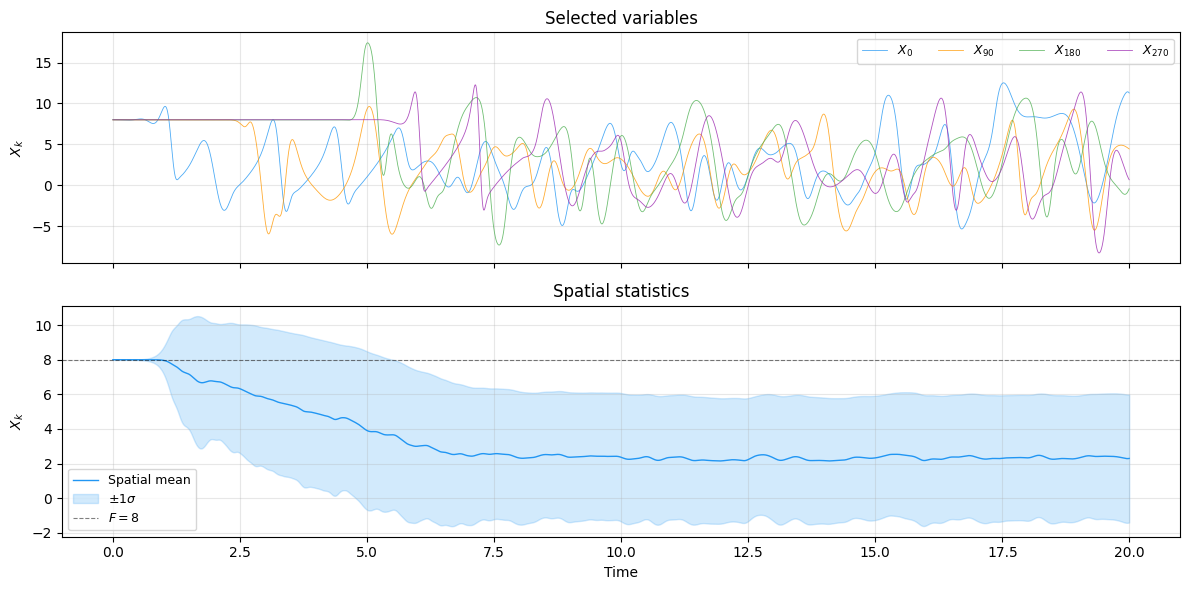

5. Diagnostics¶

model.diagnose() returns the total energy $E = \tfrac{1}{2} \sum_k X_k^2$ and the spatial mean.

diags = jax.vmap(model.diagnose)(sol.ys)

fig, axes = plt.subplots(1, 2, figsize=(12, 3.5))

axes[0].plot(ts, diags.energy, lw=0.8, color="#F44336")
axes[0].set_xlabel("Time")
axes[0].set_ylabel("Energy")
axes[0].set_title("Total energy")
axes[0].grid(True, alpha=0.3)

axes[1].plot(ts, diags.mean, lw=0.8, color="#4CAF50")
axes[1].axhline(8.0, color="k", ls="--", lw=0.8, alpha=0.5)
axes[1].set_xlabel("Time")
axes[1].set_ylabel("Mean")
axes[1].set_title("Spatial mean")
axes[1].grid(True, alpha=0.3)

plt.tight_layout()
plt.show()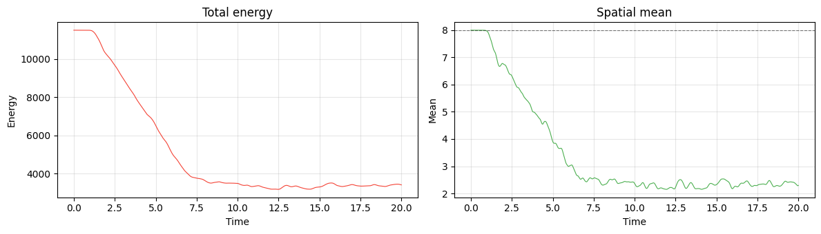

6. Forcing regimes¶

The Lorenz '96 system transitions from steady state to periodic to chaotic as $F$ increases. We compare three regimes.

F_values = [2.0, 5.0, 8.0]
regime_labels = ["$F=2$ (steady)", "$F=5$ (periodic)", "$F=8$ (chaotic)"]
regime_colors = ["#4CAF50", "#FF9800", "#F44336"]

fig, axes = plt.subplots(1, 3, figsize=(15, 4))

for ax, F_val, label, color in zip(
    axes, F_values, regime_labels, regime_colors, strict=True
):
    m = Lorenz96.create(F=F_val)
    s0 = L96State.init_state(ndim=N, noise=0.01, F=F_val)
    s = m.integrate(s0, t0=0.0, t1=20.0, dt=0.005, saveat=dfx.SaveAt(ts=ts))
    ax.imshow(
        s.ys.x,
        aspect="auto",
        origin="lower",
        cmap="RdBu_r",
        vmin=-10,
        vmax=15,
        extent=[0, N, 0, 20],
        interpolation="bilinear",
    )
    ax.set_xlabel("Variable index $k$")
    ax.set_ylabel("Time")
    ax.set_title(label, color=color, fontweight="bold")

plt.suptitle("Forcing regimes", fontsize=13)
plt.tight_layout()
plt.show()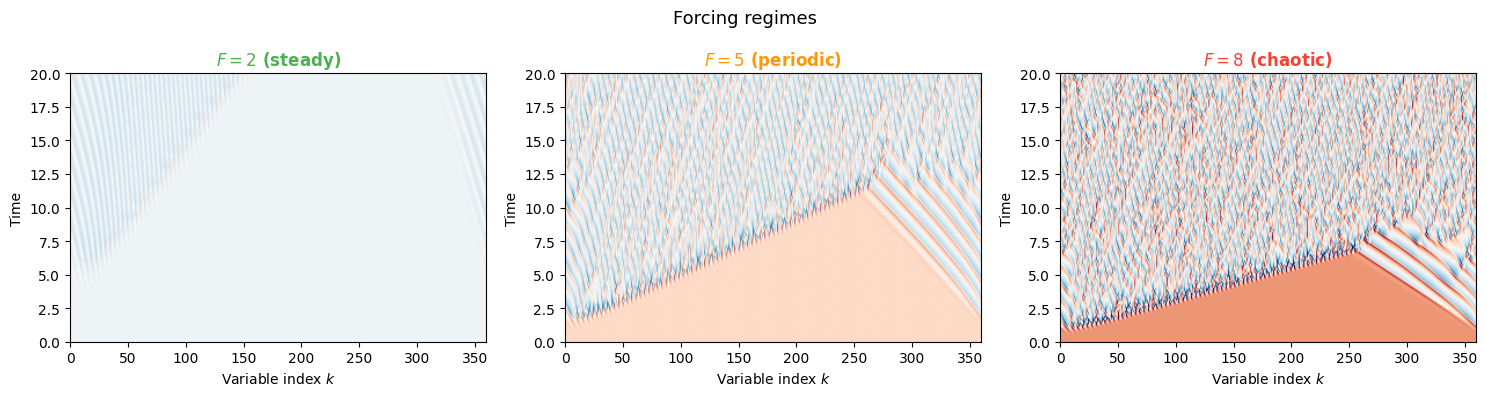

7. Adjoint methods and differentiation¶

diffrax supports several adjoint methods for backpropagating through diffeqsolve. Each trades off memory, accuracy, and speed:

Adjoint	Memory	Gradients	Use case
`RecursiveCheckpointAdjoint`	$O(\sqrt{N})$	Exact	Default
`DirectAdjoint`	$O(N)$	Exact	Short windows
`BacksolveAdjoint`	$O(1)$	Approx	Long windows
`ImplicitAdjoint`	$O(1)$	Exact	Steady states

RecursiveCheckpointAdjoint (the default) uses optimal checkpointing: re-computes forward steps from saved checkpoints, giving exact gradients with $O(\sqrt{N})$ memory.
DirectAdjoint stores the entire forward trajectory — exact but $O(N)$ memory. Also supports forward-mode AD.
BacksolveAdjoint solves the continuous adjoint ODE backwards with $O(1)$ memory. Gradients are approximate (optimize-then-discretize).
ImplicitAdjoint uses the implicit function theorem: $du^*/d\theta = -(dg/du)^{-1}\, dg/d\theta$ . Exact and $O(1)$ memory, but only for steady-state / fixed-point solves.

7a. Gradient w.r.t. parameters¶

Use case: parameter estimation. Find the forcing $F$ that minimizes a cost function over the trajectory:

\frac{\partial \mathcal{L}}{\partial F} = \int_0^T \lambda(t)^\top \frac{\partial f}{\partial F}\, dt

(2)

state0_grad = L96State.init_state(ndim=N, noise=0.01, F=8.0)


@eqx.filter_grad
def grad_params(model):
    sol = model.integrate(state0_grad, t0=0.0, t1=1.0, dt=0.005)
    return jnp.sum(sol.ys.x**2)


grads_theta = grad_params(model)
print("--- Gradient w.r.t. parameters ---")
print(f"  dL/dF = {grads_theta.params.F:.4f}")

--- Gradient w.r.t. parameters ---
  dL/dF = 3630.4766

7b. Gradient w.r.t. initial state¶

Use case: 4D-Var data assimilation. Find the initial condition $\mathbf{X}_0$ that best fits observations. The gradient is the adjoint state at $t = 0$ :

\frac{\partial \mathcal{L}}{\partial \mathbf{X}_0} = \lambda(0)

(3)

def loss_state(state0):
    sol = model.integrate(state0, t0=0.0, t1=1.0, dt=0.005)
    return jnp.sum(sol.ys.x**2)


grads_u0 = jax.grad(loss_state)(state0_grad)

print("--- Gradient w.r.t. initial state ---")
print(f"  dL/d(X0) shape: {grads_u0.x.shape}")
print(f"  dL/d(X0) norm:  {jnp.linalg.norm(grads_u0.x):.4f}")
print(f"  dL/d(X0)[:5]:   {grads_u0.x[:5]}")

--- Gradient w.r.t. initial state ---
  dL/d(X0) shape: (360,)
  dL/d(X0) norm:  4228.1538
  dL/d(X0)[:5]:   [-1638.6827   -413.43512  1382.2256   1065.4902   -724.1401 ]

7c. Joint gradient — parameters and state¶

Use case: weak-constraint 4D-Var / bi-level optimization. Simultaneously optimize the initial condition and model parameters.

def loss_joint(state0, model):
    sol = model.integrate(state0, t0=0.0, t1=1.0, dt=0.005)
    return jnp.sum(sol.ys.x**2)


grads_u0_joint, grads_model_joint = jax.grad(loss_joint, argnums=(0, 1))(
    state0_grad, model
)

print("--- Joint gradient ---")
print(f"  dL/dF         = {grads_model_joint.params.F:.4f}")
print(f"  dL/d(X0) norm = {jnp.linalg.norm(grads_u0_joint.x):.4f}")

--- Joint gradient ---
  dL/dF         = 3630.4766
  dL/d(X0) norm = 4228.1538

7d. Comparing adjoint methods¶

We time RecursiveCheckpointAdjoint vs DirectAdjoint. BacksolveAdjoint requires a different API pattern (explicit args to diffeqsolve, not via closure) — see the diffrax docs.

import time


def timed_grad(adjoint, label):
    @eqx.filter_grad
    def fn(model):
        sol = model.integrate(state0_grad, t0=0.0, t1=1.0, dt=0.005, adjoint=adjoint)
        return jnp.sum(sol.ys.x**2)

    g = fn(model)
    jax.block_until_ready(g.params.F)
    t_start = time.perf_counter()
    g = fn(model)
    jax.block_until_ready(g.params.F)
    elapsed = time.perf_counter() - t_start
    print(f"  {label:25s}  dL/dF={g.params.F:.2f}  ({elapsed:.4f}s)")


print("--- Adjoint method comparison ---")
timed_grad(dfx.RecursiveCheckpointAdjoint(), "RecursiveCheckpoint")
timed_grad(dfx.DirectAdjoint(), "Direct")

--- Adjoint method comparison ---

  RecursiveCheckpoint        dL/dF=3630.48  (3.6390s)

  Direct                     dL/dF=3630.47  (2.5357s)

8. Ensemble forecast divergence¶

We launch 30 ensemble members from perturbed initial conditions and measure the ensemble spread over time — the hallmark of deterministic chaos.

n_ensemble = 30
key = jrandom.PRNGKey(0)
perturb = 0.01 * jrandom.normal(key, shape=(n_ensemble, N))
x0_base = 8.0 * jnp.ones(N)
ensemble_states = L96State(x=x0_base[None, :] + perturb)

ts_ens = jnp.arange(0.0, 10.0, 0.05)


def integrate_one(state0):
    return model.integrate(
        state0,
        t0=0.0,
        t1=10.0,
        dt=0.005,
        saveat=dfx.SaveAt(ts=ts_ens),
    )


ensemble_sol = eqx.filter_vmap(integrate_one)(ensemble_states)

# Compute ensemble spread (RMSE relative to ensemble mean)
ens_mean = jnp.mean(ensemble_sol.ys.x, axis=0)  # (T, N)
spread = jnp.sqrt(
    jnp.mean((ensemble_sol.ys.x - ens_mean[None, :, :]) ** 2, axis=(0, 2))
)

fig, axes = plt.subplots(1, 2, figsize=(13, 4))

# Left: spaghetti plot for variable 0
ax = axes[0]
for j in range(n_ensemble):
    ax.plot(ts_ens, ensemble_sol.ys.x[j, :, 0], lw=0.3, alpha=0.5, color="#2196F3")
ax.plot(ts_ens, ens_mean[:, 0], lw=2, color="#F44336", label="Ensemble mean")
ax.set_xlabel("Time")
ax.set_ylabel("$X_0$")
ax.set_title("Spaghetti plot — $X_0$")
ax.legend(fontsize=9)
ax.grid(True, alpha=0.3)

# Right: ensemble spread
ax = axes[1]
ax.plot(ts_ens, spread, lw=1.5, color="#9C27B0")
ax.set_xlabel("Time")
ax.set_ylabel("RMSE spread")
ax.set_title("Ensemble spread growth")
ax.grid(True, alpha=0.3)

plt.tight_layout()
plt.show()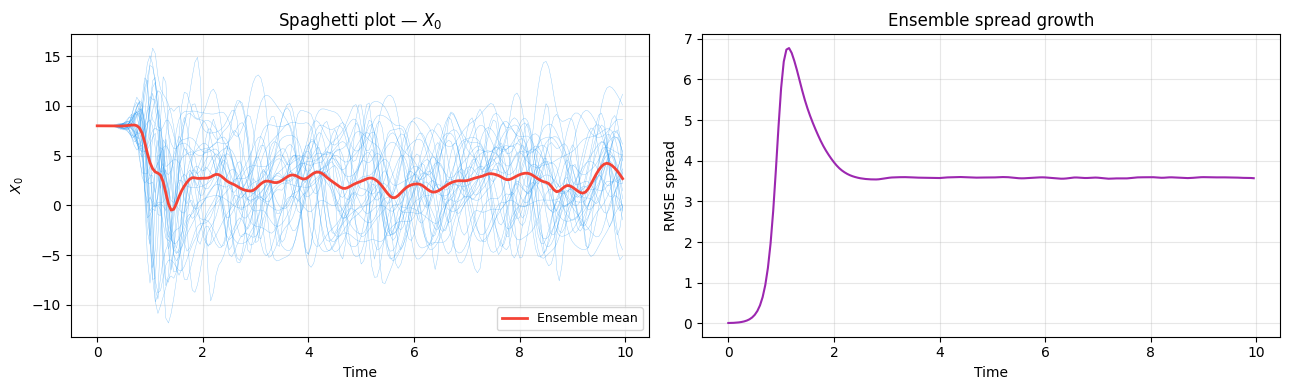

Summary¶

Concept	somax API
Create a model	`Lorenz96.create(F=8.0)`
Initial condition	`L96State.init_state(ndim=40, F=8.0)`
Forward simulation	`model.integrate(state0, t0, t1, dt, saveat=...)`
Diagnostics	`model.diagnose(state)` — energy, mean
Grad w.r.t. params	`eqx.filter_grad(loss)(model)` — dL/dF
Grad w.r.t. state	`jax.grad(loss)(state0)` — dL/dX0
Joint grad	`jax.grad(loss, argnums=(0, 1))(state0, model)`
Ensemble	`eqx.filter_vmap(integrate_one)(batch_states)`

Key takeaways:

$F = 8$ produces fully developed chaos with a doubling time of ~0.42 time units
The Hovmoller diagram reveals eastward-propagating wave packets
Ensemble spread saturates after ~4 time units (the predictability horizon)