Lorenz '96 Two-Tier — Slow-Fast Multiscale Chaos - somax: Simple Ocean Models in JAX

The two-tier Lorenz '96 system couples a set of slow large-scale variables $X_k$ to a set of fast small-scale variables $Y_{j,k}$ . It is the standard test bed for studying multiscale dynamics, sub-grid parameterization, and stochastic closures.

What you’ll learn:

How slow and fast variables interact through coupling
How the Hovmoller diagram reveals the multiscale structure
How coupling strength controls fast-variable activity
How to differentiate through a multiscale simulation

Background¶

The system consists of $D_x$ slow variables $X_k$ and $D_y \times D_x$ fast variables $Y_{j,k}$ :

\frac{dX_k}{dt} = (X_{k+1} - X_{k-2})\, X_{k-1} - X_k + F - \frac{hc}{b} \sum_{j=1}^{D_y} Y_{j,k}

(1)

\frac{dY_{j,k}}{dt} = cb\,(Y_{j+1,k} - Y_{j-2,k})\, Y_{j-1,k} - c\, Y_{j,k} + \frac{hc}{b}\, X_k

(2)

The key parameters are:

Parameter	Role	Standard value
$F$	External forcing on slow variables	18
$h$	Coupling coefficient	1
$b$	Amplitude ratio (fast / slow)	10
$c$	Time-scale ratio (fast / slow)	10

The fast variables evolve $c = 10$ times faster than the slow variables and have $b = 10$ times smaller amplitude. The coupling term $hc/b$ transfers energy between scales.

from __future__ import annotations

import diffrax as dfx
import einops
import equinox as eqx
import jax
import jax.numpy as jnp
import jax.random as jrandom
import matplotlib.pyplot as plt

from somax.models import L96TState, Lorenz96t

1. Create the model¶

We use $D_x = 36$ slow variables and $D_y = 10$ fast variables per slow variable (360 fast variables total).

Dx, Dy = 36, 10
model = Lorenz96t.create(F=18.0, h=1.0, b=10.0, c=10.0)
print(model)

Lorenz96t(
  params=L96TParams(F=weak_f32[], h=weak_f32[], b=weak_f32[], c=weak_f32[])
)

2. Forward simulation¶

The fast variables require a small time step. We integrate for 2 time units (roughly 10 days in the L96 convention) and save at a moderate output rate.

state0 = L96TState.init_state(ndims=(Dx, Dy), noise=0.01, b=10.0)

t0, t1, dt = 0.0, 2.0, 0.0005
ts = jnp.arange(t0, t1, 0.005)  # save every 0.005

sol = model.integrate(
    state0,
    t0=t0,
    t1=t1,
    dt=dt,
    saveat=dfx.SaveAt(ts=ts),
)

print(f"Slow variables: {sol.ys.x.shape}")  # (T, Dx)
print(f"Fast variables: {sol.ys.y.shape}")  # (T, Dy*Dx)

Slow variables: (400, 36)
Fast variables: (400, 360)

3. Slow and fast time series¶

The slow variables look like noisy oscillations (similar to standard L96), while the fast variables show rapid fluctuations modulated by the slow-variable envelope.

colors_slow = ["#2196F3", "#FF9800", "#4CAF50", "#9C27B0"]
colors_fast = ["#F44336", "#00BCD4", "#795548"]

fig, axes = plt.subplots(2, 1, figsize=(13, 6), sharex=True)

# Slow variables
ax = axes[0]
for idx, c in zip([0, 9, 18, 27], colors_slow, strict=True):
    ax.plot(ts, sol.ys.x[:, idx], lw=0.8, color=c, label=f"$X_{{{idx}}}$")
ax.set_ylabel("$X_k$")
ax.set_title("Slow variables")
ax.legend(fontsize=9, ncol=4)
ax.grid(True, alpha=0.3)

# Fast variables (a few from different slow-variable sectors)
ax = axes[1]
y_2d = einops.rearrange(sol.ys.y, "T (Dy Dx) -> T Dy Dx", Dy=Dy, Dx=Dx)
for j_idx, k_idx, c in zip([0, 3, 7], [0, 12, 24], colors_fast, strict=True):
    ax.plot(
        ts,
        y_2d[:, j_idx, k_idx],
        lw=0.4,
        alpha=0.8,
        color=c,
        label=f"$Y_{{{j_idx},{k_idx}}}$",
    )
ax.set_xlabel("Time")
ax.set_ylabel("$Y_{j,k}$")
ax.set_title("Fast variables")
ax.legend(fontsize=9, ncol=3)
ax.grid(True, alpha=0.3)

plt.tight_layout()
plt.show()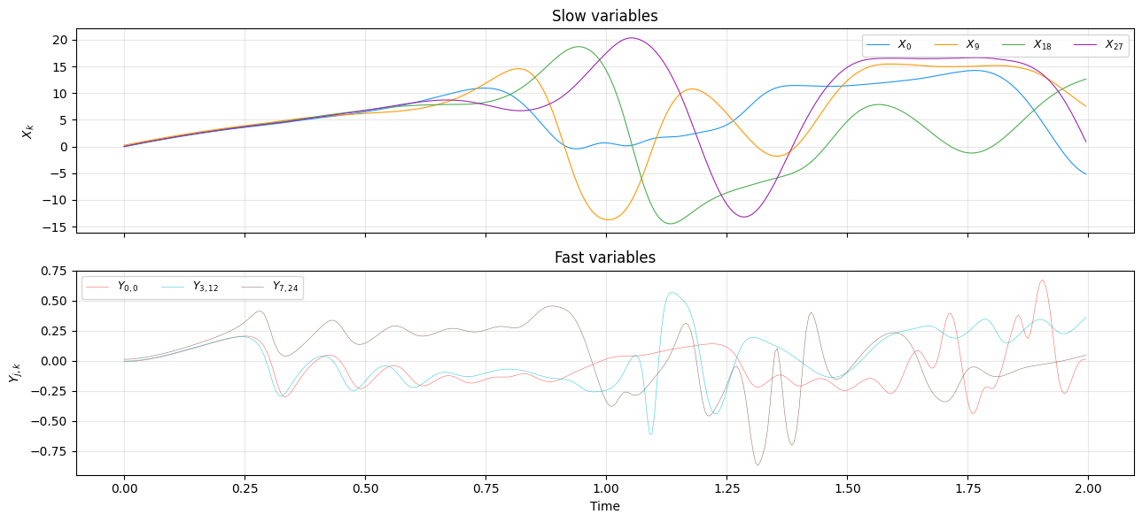

4. Hovmoller diagrams — slow vs fast¶

The slow-variable Hovmoller shows the familiar wave propagation. The fast-variable Hovmoller (averaged over the $j$ -index) reveals the small-scale activity modulated by the large-scale pattern.

y_2d_full = einops.rearrange(sol.ys.y, "T (Dy Dx) -> T Dy Dx", Dy=Dy, Dx=Dx)
y_mean_over_j = jnp.mean(y_2d_full, axis=1)  # (T, Dx)

fig, axes = plt.subplots(1, 2, figsize=(14, 5))

# Slow
im0 = axes[0].imshow(
    sol.ys.x,
    aspect="auto",
    origin="lower",
    cmap="RdBu_r",
    extent=[0, Dx, float(ts[0]), float(ts[-1])],
    interpolation="bilinear",
)
axes[0].set_xlabel("Slow variable index $k$")
axes[0].set_ylabel("Time")
axes[0].set_title("Slow variables $X_k$")
plt.colorbar(im0, ax=axes[0], label="$X_k$")

# Fast (j-averaged)
im1 = axes[1].imshow(
    y_mean_over_j,
    aspect="auto",
    origin="lower",
    cmap="PuOr_r",
    extent=[0, Dx, float(ts[0]), float(ts[-1])],
    interpolation="bilinear",
)
axes[1].set_xlabel("Slow variable index $k$")
axes[1].set_ylabel("Time")
axes[1].set_title(r"Fast variables $\langle Y_{j,k} \rangle_j$")
plt.colorbar(im1, ax=axes[1], label=r"$\langle Y \rangle_j$")

plt.tight_layout()
plt.show()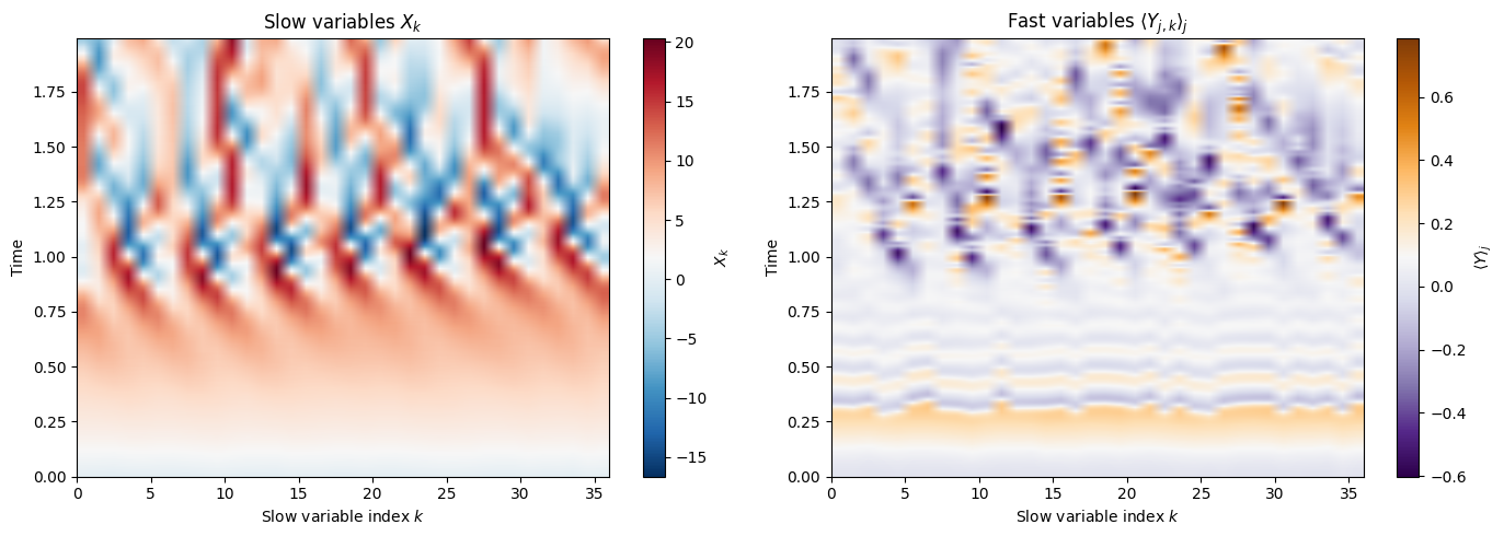

5. Energy partition¶

The total energy splits between slow and fast components. The fast variables carry less energy per mode but there are $D_y$ times as many of them.

slow_energy = 0.5 * jnp.sum(sol.ys.x**2, axis=1)
fast_energy = 0.5 * jnp.sum(sol.ys.y**2, axis=1)

fig, ax = plt.subplots(figsize=(12, 3.5))
ax.plot(ts, slow_energy, lw=1, color="#2196F3", label="Slow energy")
ax.plot(ts, fast_energy, lw=1, color="#F44336", label="Fast energy")
ax.plot(ts, slow_energy + fast_energy, lw=1.5, color="k", ls="--", label="Total")
ax.set_xlabel("Time")
ax.set_ylabel("Energy")
ax.set_title("Energy partition between slow and fast variables")
ax.legend(fontsize=9)
ax.grid(True, alpha=0.3)
plt.tight_layout()
plt.show()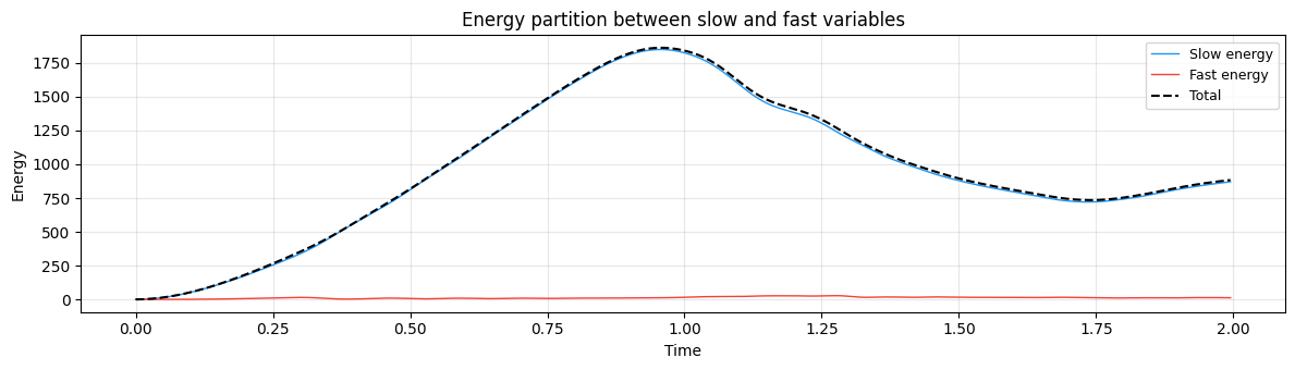

6. Coupling strength¶

The coupling coefficient $h$ controls how strongly the fast variables feed back onto the slow variables. We compare three regimes: uncoupled ( $h = 0$ ), weakly coupled ( $h = 0.5$ ), and strongly coupled ( $h = 1$ ).

h_values = [0.0, 0.5, 1.0]
h_labels = ["$h=0$ (uncoupled)", "$h=0.5$ (weak)", "$h=1$ (strong)"]
h_colors = ["#4CAF50", "#FF9800", "#F44336"]

fig, axes = plt.subplots(1, 3, figsize=(15, 4))

for ax, h_val, label, color in zip(axes, h_values, h_labels, h_colors, strict=True):
    m = Lorenz96t.create(F=18.0, h=h_val, b=10.0, c=10.0)
    s0 = L96TState.init_state(ndims=(Dx, Dy), noise=0.01, b=10.0)
    s = m.integrate(s0, t0=0.0, t1=2.0, dt=0.0005, saveat=dfx.SaveAt(ts=ts))
    ax.imshow(
        s.ys.x,
        aspect="auto",
        origin="lower",
        cmap="RdBu_r",
        extent=[0, Dx, 0, 2],
        interpolation="bilinear",
    )
    ax.set_xlabel("Slow variable index $k$")
    ax.set_ylabel("Time")
    ax.set_title(label, color=color, fontweight="bold")

plt.suptitle("Coupling regimes — slow variables", fontsize=13)
plt.tight_layout()
plt.show()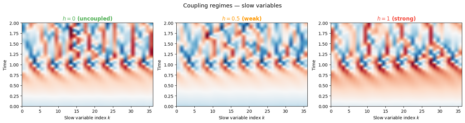

7. Adjoint methods and differentiation¶

Differentiating through a stiff multiscale ODE is more challenging than a single-scale system because the fast variables demand many time steps. diffrax provides three adjoint methods:

Adjoint	Memory	Gradients	Use case
`RecursiveCheckpointAdjoint`	$O(\sqrt{N})$	Exact	Default
`DirectAdjoint`	$O(N)$	Exact	Short windows
`BacksolveAdjoint`	$O(1)$	Approx	Long windows
`ImplicitAdjoint`	$O(1)$	Exact	Steady states

RecursiveCheckpointAdjoint (the default) uses optimal checkpointing: re-computes forward steps from saved checkpoints, giving exact gradients with $O(\sqrt{N})$ memory.
DirectAdjoint stores the entire forward trajectory — exact but $O(N)$ memory.
BacksolveAdjoint solves the continuous adjoint ODE backwards with $O(1)$ memory. Gradients are approximate.
ImplicitAdjoint uses the implicit function theorem: $du^*/d\theta = -(dg/du)^{-1}\, dg/d\theta$ . Exact and $O(1)$ memory, but only for steady-state / fixed-point solves.

For this system with $dt = 5 \times 10^{-4}$ , even a short window of $T = 0.5$ requires 1000 steps. RecursiveCheckpointAdjoint is the best default because it avoids storing all 1000 forward states.

7a. Gradient w.r.t. parameters¶

Use case: parameter estimation. All four coupling parameters $(F, h, b, c)$ are differentiable. The adjoint equations are:

\frac{\partial \mathcal{L}}{\partial \theta} = \int_0^T \lambda(t)^\top \frac{\partial f}{\partial \theta}\, dt, \qquad \theta = (F, h, b, c)

(3)

state0_grad = L96TState.init_state(ndims=(Dx, Dy), noise=0.01, b=10.0)


@eqx.filter_grad
def grad_params(model):
    sol = model.integrate(state0_grad, t0=0.0, t1=0.5, dt=0.0005)
    return jnp.sum(sol.ys.x**2)


grads_theta = grad_params(model)
print("--- Gradient w.r.t. parameters ---")
print(f"  dL/dF = {grads_theta.params.F:.4f}")
print(f"  dL/dh = {grads_theta.params.h:.4f}")
print(f"  dL/db = {grads_theta.params.b:.4f}")
print(f"  dL/dc = {grads_theta.params.c:.4f}")

--- Gradient w.r.t. parameters ---
  dL/dF = 193.4378
  dL/dh = -128.4092
  dL/db = 39.7463
  dL/dc = 0.3340

7b. Gradient w.r.t. initial state¶

Use case: 4D-Var. Find the initial condition $(\mathbf{X}_0, \mathbf{Y}_0)$ that best fits observations. The gradient is the adjoint state at $t = 0$ :

\frac{\partial \mathcal{L}}{\partial \mathbf{u}_0} = \lambda(0), \qquad \mathbf{u}_0 = (\mathbf{X}_0, \mathbf{Y}_0)

(4)

In practice one often assimilates only the slow variables and lets the fast variables spin up.

def loss_state(state0):
    sol = model.integrate(state0, t0=0.0, t1=0.5, dt=0.0005)
    return jnp.sum(sol.ys.x**2)


grads_u0 = jax.grad(loss_state)(state0_grad)

print("--- Gradient w.r.t. initial state ---")
print(f"  dL/d(X0) shape: {grads_u0.x.shape}")
print(f"  dL/d(X0) norm:  {jnp.linalg.norm(grads_u0.x):.4f}")
print(f"  dL/d(Y0) shape: {grads_u0.y.shape}")
print(f"  dL/d(Y0) norm:  {jnp.linalg.norm(grads_u0.y):.4f}")

--- Gradient w.r.t. initial state ---
  dL/d(X0) shape: (36,)

  dL/d(X0) norm:  52.9541
  dL/d(Y0) shape: (360,)
  dL/d(Y0) norm:  1425.0918

7c. Joint gradient — parameters and state¶

Use case: weak-constraint 4D-Var. Simultaneously optimize the initial condition and all coupling parameters.

def loss_joint(state0, model):
    sol = model.integrate(state0, t0=0.0, t1=0.5, dt=0.0005)
    return jnp.sum(sol.ys.x**2)


grads_u0_joint, grads_model_joint = jax.grad(loss_joint, argnums=(0, 1))(
    state0_grad, model
)

print("--- Joint gradient ---")
print(f"  dL/dF         = {grads_model_joint.params.F:.4f}")
print(f"  dL/dh         = {grads_model_joint.params.h:.4f}")
print(f"  dL/d(X0) norm = {jnp.linalg.norm(grads_u0_joint.x):.4f}")
print(f"  dL/d(Y0) norm = {jnp.linalg.norm(grads_u0_joint.y):.4f}")

--- Joint gradient ---
  dL/dF         = 193.4378
  dL/dh         = -128.4092
  dL/d(X0) norm = 52.9541
  dL/d(Y0) norm = 1425.0918

8. Ensemble divergence¶

We launch 20 ensemble members and track how the slow-variable spread grows over time.

n_ensemble = 20
key = jrandom.PRNGKey(7)
key_x, key_y = jrandom.split(key)

x0 = 0.1 * jrandom.normal(key_x, shape=(n_ensemble, Dx))
y0 = 0.01 * jrandom.normal(key_y, shape=(n_ensemble, Dy * Dx))
ensemble_states = L96TState(x=x0, y=y0)

ts_ens = jnp.arange(0.0, 2.0, 0.005)


def integrate_one(state0):
    return model.integrate(
        state0,
        t0=0.0,
        t1=2.0,
        dt=0.0005,
        saveat=dfx.SaveAt(ts=ts_ens),
    )


ensemble_sol = eqx.filter_vmap(integrate_one)(ensemble_states)

# Slow-variable ensemble spread
ens_mean_x = jnp.mean(ensemble_sol.ys.x, axis=0)  # (T, Dx)
spread_x = jnp.sqrt(
    jnp.mean((ensemble_sol.ys.x - ens_mean_x[None, :, :]) ** 2, axis=(0, 2))
)

fig, axes = plt.subplots(1, 2, figsize=(13, 4))

# Spaghetti — slow variable 0
ax = axes[0]
for j in range(n_ensemble):
    ax.plot(
        ts_ens,
        ensemble_sol.ys.x[j, :, 0],
        lw=0.4,
        alpha=0.5,
        color="#2196F3",
    )
ax.plot(ts_ens, ens_mean_x[:, 0], lw=2, color="#F44336", label="Ensemble mean")
ax.set_xlabel("Time")
ax.set_ylabel("$X_0$")
ax.set_title("Spaghetti plot — slow $X_0$")
ax.legend(fontsize=9)
ax.grid(True, alpha=0.3)

# Spread
ax = axes[1]
ax.plot(ts_ens, spread_x, lw=1.5, color="#9C27B0")
ax.set_xlabel("Time")
ax.set_ylabel("RMSE spread")
ax.set_title("Slow-variable ensemble spread")
ax.grid(True, alpha=0.3)

plt.tight_layout()
plt.show()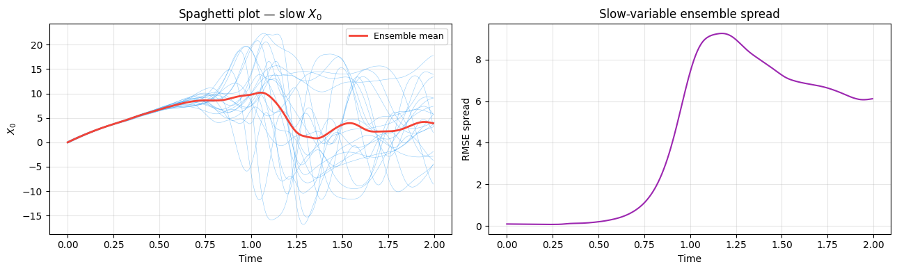

Summary¶

Concept	somax API
Create a model	`Lorenz96t.create(F=18, h=1, b=10, c=10)`
Initial condition	`L96TState.init_state(ndims=(Dx, Dy))`
Forward simulation	`model.integrate(state0, t0, t1, dt)`
Grad w.r.t. params	`eqx.filter_grad(loss)(model)` — all 4 params
Grad w.r.t. state	`jax.grad(loss)(state0)` — dL/d(X0, Y0)
Joint grad	`jax.grad(loss, argnums=(0, 1))(state0, model)`
Ensemble	`eqx.filter_vmap(integrate_one)(batch_states)`

Key takeaways:

The fast variables evolve $c = 10$ times faster than the slow variables, requiring a small time step ( $dt \approx 5 \times 10^{-4}$ )
Coupling ( $h > 0$ ) feeds fast-variable energy back into the slow dynamics, modifying the large-scale attractor
This system is the standard test bed for learned sub-grid parameterizations (replacing the fast variables with a closure)