Capacitance Solver Guide¶

Practical guide for solving elliptic PDEs on masked/irregular domains using the capacitance matrix method in SpectralDiffX.

When to Use the Capacitance Solver¶

You have a masked domain -- an ocean basin with coastlines, a room with obstacles, or any region that is a subset of a rectangle. The fast spectral solvers (DST/DCT/FFT) require a full rectangle. The capacitance solver extends them to irregular domains by correcting for the boundary mismatch.

Use the capacitance solver when:

Your domain is a subset of a rectangle defined by a boolean mask
You want the speed of spectral methods (not iterative CG)
The boundary perimeter is manageable (N_b < ~1000 points)

The Two-Phase Workflow¶

The capacitance method splits into an offline phase (expensive, done once) and an online phase (cheap, done many times).

import numpy as np
from spectraldiffx import build_capacitance_solver

Ny, Nx = 64, 64
j, i = np.mgrid[0:Ny, 0:Nx]
mask = (j - Ny / 2) ** 2 + (i - Nx / 2) ** 2 < (0.4 * Nx) ** 2  # circular basin
rhs = np.where(mask, 1.0, 0.0)

# ----- Offline: build the solver (N_b spectral solves) -----
solver = build_capacitance_solver(
    mask,               # bool array [Ny, Nx]: True = interior
    dx=1.0,
    dy=1.0,
    lambda_=0.0,        # 0 for Poisson, >0 for Helmholtz
    base_bc="dst",      # "fft", "dst", or "dct"
)

# ----- Online: solve for any rhs (fast) -----
psi = solver(rhs)       # rhs is [Ny, Nx], returns [Ny, Nx]

The solver object is an eqx.Module (a pure pytree). It wraps a gaussx.MaskedOperator holding the LU-factorised N_b x N_b capacitance matrix, so the online solve is two rectangular spectral solves plus an N_b x N_b back-substitution.

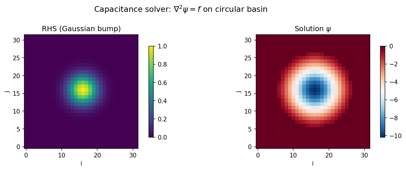
Capacitance solver on a circular ocean basin. Left: mask with inner-boundary points (red). Center: RHS (ones inside mask). Right: solution psi.

Building a Mask¶

The mask is a 2-D boolean array where True marks interior (fluid) cells and False marks exterior (land/wall) cells.

Example: circular basin in a rectangle¶

import numpy as np

Ny, Nx = 64, 64
j, i = np.mgrid[0:Ny, 0:Nx]
radius = 0.4 * min(Ny, Nx)
mask = ((j - Ny / 2)**2 + (i - Nx / 2)**2) < radius**2

Example: rectangle with a rectangular obstacle¶

mask = np.ones((Ny, Nx), dtype=bool)
mask[20:30, 25:40] = False  # obstacle

Example: L-shaped domain¶

mask = np.ones((Ny, Nx), dtype=bool)
mask[Ny // 2:, :Nx // 2] = False  # remove lower-left quadrant

Inner boundary detection is automatic

You do not need to mark boundary points explicitly. The solver automatically detects inner-boundary cells as mask-interior cells that are 4-connected to at least one exterior cell. With base_bc="fft" the neighbourhood wraps around the periodic rectangle, so wet cells on the rectangle edge whose wrapped neighbour is dry are treated as boundary.

Choosing `base_bc`¶

The base_bc parameter selects which rectangular spectral solver to use as the "base" for the capacitance correction:

`base_bc`	Base solver	Rectangle BCs	Notes
`"fft"`	`solve_helmholtz_fft`	Periodic	Default. Good general choice.
`"dst"`	`solve_helmholtz_dst`	Dirichlet	Natural if mask boundary touches rectangle edges. May give fewer boundary points near edges.
`"dct"`	`solve_helmholtz_dct`	Neumann	Use if the outer rectangle should have zero-flux.

All three produce the same result on the masked interior (the capacitance correction enforces psi = 0 at inner-boundary points regardless of the rectangular BC). The choice affects:

Number of boundary points: DST may reduce N_b when the mask touches rectangle edges (since DST already enforces zero there)
Null mode handling: FFT and DCT have a null (constant) mode for Poisson; DST does not. The solver handles it automatically: the constant null vector enters the capacitance system, so the PDE holds exactly in the interior for every base (earlier versions left a uniform residual here)

When in doubt, use base_bc=\"dst\"

For bounded physical domains where the solution is zero on the outer boundary, DST is the most natural choice and often gives the smallest N_b.

Memory and Performance¶

The offline phase performs N_b spectral solves (one column of the capacitance matrix each) and keeps only the LU factors of the N_b x N_b capacitance matrix; no Green's-function table is stored. The online phase is two spectral solves plus an N_b x N_b back-substitution.

Measured at 256 x 256 with a circular mask (N_b = 520, base_bc="fft", float64, CPU): build 1.5 s, 4 ms per solve, 3.5 MB stored. Memory grows as O(N_b² + Ny·Nx) and the offline time as O(N_b · Ny·Nx · log(Ny·Nx)).

Rule of thumb: N_b ~ O(perimeter)

The number of inner-boundary points scales with the perimeter of the masked region, not its area. A 64x64 circular domain has N_b ~ 200 (circumference ~ 2pi25). A 64x64 square domain with one hole has N_b equal to the hole's perimeter.

Code Example: Ocean Basin¶

A complete worked example: create a circular ocean mask, build the capacitance solver, solve a Poisson equation, and verify.

import jax
import jax.numpy as jnp
import numpy as np
from spectraldiffx import build_capacitance_solver

jax.config.update("jax_enable_x64", True)

# --- Grid setup ---
Ny, Nx = 64, 64
dx, dy = 1.0, 1.0

# --- Create a circular ocean mask ---
j, i = np.mgrid[0:Ny, 0:Nx]
center_j, center_i = Ny / 2, Nx / 2
radius = 0.35 * min(Ny, Nx)
mask = ((j - center_j)**2 + (i - center_i)**2) < radius**2

print(f"Mask shape: {mask.shape}")
print(f"Interior points: {mask.sum()}")

# --- Build the solver (offline, one-time) ---
solver = build_capacitance_solver(
    mask,
    dx=dx,
    dy=dy,
    lambda_=0.0,     # Poisson equation
    base_bc="dst",   # Dirichlet rectangle
)
interior = np.zeros(mask.size, dtype=bool)
interior[np.asarray(solver.interior_indices)] = True
boundary = mask & ~interior.reshape(mask.shape)  # inner-boundary cells
print(f"Boundary points (N_b): {boundary.sum()}")

# --- Create a source term ---
j_jax = jnp.arange(Ny)[:, None]
i_jax = jnp.arange(Nx)[None, :]
rhs = jnp.sin(jnp.pi * (j_jax - center_j) / radius) * \
      jnp.sin(jnp.pi * (i_jax - center_i) / radius)
rhs = rhs * jnp.array(mask, dtype=float)  # zero outside mask

# --- Solve (online, fast) ---
psi = solver(rhs)

# --- Verify: psi should be ~0 at boundary points ---
boundary_values = psi[boundary]
print(f"Max |psi| at boundary: {jnp.max(jnp.abs(boundary_values)):.2e}")
# Should be ~1e-14 or smaller with float64

# --- Mask the exterior for visualization ---
psi_masked = psi * jnp.array(mask, dtype=float)

Batched Solves¶

Once built, the solver works with jax.vmap for batched right-hand sides:

import jax

# Stack of 10 right-hand sides
rhs_batch = jnp.stack([rhs * (k + 1) for k in range(10)])  # [10, Ny, Nx]

# vmap the online solve
solve_batch = jax.vmap(solver)
psi_batch = solve_batch(rhs_batch)  # [10, Ny, Nx]

The offline precomputation is shared across all batch elements -- only the cheap online solve is repeated.

Limitations¶

Large N_b (> ~1000): consider iterative solvers

The capacitance matrix is N_b x N_b (dense) and the build needs N_b spectral solves. When N_b exceeds a few thousand, memory and offline time become significant. For very fine grids or domains with long, convoluted boundaries, consider using an iterative solver (e.g., preconditioned CG in finitevolX) instead.

The capacitance matrix is dense

Its LU factorisation is O(N_b^3) at build time, but it only happens once.

Mask must have interior/exterior structure

build_capacitance_solver raises a ValueError if the mask is all True (no exterior cells: just use the rectangular spectral solver directly), all False (no wet cells), or so thin that every wet cell is on the inner boundary (no interior unknowns).

Homogeneous BCs only

The capacitance method enforces psi = 0 at all inner-boundary points. For inhomogeneous Dirichlet BCs (psi = g on the boundary), you can subtract a known function that satisfies the boundary data and solve for the remainder.