Mixed Per-Axis Boundary Conditions¶

The solve_helmholtz_2d solver supports different boundary conditions on each axis, enabling problems that the monolithic solvers (solve_helmholtz_dst, solve_helmholtz_fft, etc.) cannot handle.

This notebook demonstrates three physically motivated scenarios:

Scenario	BC in x	BC in y	Physical analogy
Channel flow	Periodic	Dirichlet	Poiseuille-like pressure solve
Heated plate	Dirichlet	Neumann	Hot/cold walls, insulated top/bottom
Half-pipe	Dirichlet left + Neumann right	Dirichlet	Inlet wall + symmetry plane

In [ ]:

from pathlib import Path

import jax
import jax.numpy as jnp
import matplotlib
import matplotlib.pyplot as plt
import numpy as np

matplotlib.use("Agg")
jax.config.update("jax_enable_x64", True)

from spectraldiffx import MixedBCHelmholtzSolver2D, solve_helmholtz_2d, solve_poisson_2d

IMG_DIR = (
    Path(__file__).resolve().parent.parent / "docs" / "images" / "mixed_bc_solvers"
)
IMG_DIR.mkdir(parents=True, exist_ok=True)

from pathlib import Path import jax import jax.numpy as jnp import matplotlib import matplotlib.pyplot as plt import numpy as np matplotlib.use("Agg") jax.config.update("jax_enable_x64", True) from spectraldiffx import MixedBCHelmholtzSolver2D, solve_helmholtz_2d, solve_poisson_2d IMG_DIR = ( Path(__file__).resolve().parent.parent / "docs" / "images" / "mixed_bc_solvers" ) IMG_DIR.mkdir(parents=True, exist_ok=True)

1. Channel Flow: Periodic-x, Dirichlet-y¶

A common setup in CFD: the domain is periodic in the streamwise ($x$) direction and bounded by walls in the cross-stream ($y$) direction. We solve the Poisson equation $\nabla^2 \psi = f$ with:

• $x$: periodic (FFT)
• $y$: $\psi = 0$ on both walls (Dirichlet, DST-I)

The source term is a single Fourier-sine mode: $f(x, y) = \sin(2\pi x / L_x) \sin(\pi y / L_y)$.

In [ ]:

Nx, Ny = 64, 32
Lx, Ly = 2.0, 1.0
dx, dy = Lx / Nx, Ly / (Ny + 1)

# Grid points
x = np.arange(Nx) * dx  # periodic
y = np.linspace(dy, Ly - dy, Ny)  # interior (Dirichlet)
X, Y = np.meshgrid(x, y)

# Source term: sin(2*pi*x/Lx) * sin(pi*y/Ly)
kx, ky = 2 * np.pi / Lx, np.pi / Ly
rhs = jnp.array(np.sin(kx * X) * np.sin(ky * Y))

# Exact solution: psi = -f / (kx^2 + ky^2)
psi_exact = -np.sin(kx * X) * np.sin(ky * Y) / (kx**2 + ky**2)

# Solve with mixed BCs
psi = solve_poisson_2d(rhs, dx, dy, bc_x="periodic", bc_y="dirichlet")
psi_np = np.array(psi)

fig, axes = plt.subplots(1, 3, figsize=(15, 4), constrained_layout=True)

# Source term
im0 = axes[0].pcolormesh(X, Y, np.array(rhs), cmap="RdBu_r", shading="auto")
axes[0].set_title("Source $f(x, y)$")
axes[0].set_xlabel("$x$")
axes[0].set_ylabel("$y$")
fig.colorbar(im0, ax=axes[0], shrink=0.8)

# Solution
im1 = axes[1].pcolormesh(X, Y, psi_np, cmap="RdBu_r", shading="auto")
axes[1].set_title("Solution $\\psi(x, y)$")
axes[1].set_xlabel("$x$")
fig.colorbar(im1, ax=axes[1], shrink=0.8)

# Error
error = np.abs(psi_np - psi_exact)
im2 = axes[2].pcolormesh(X, Y, error, cmap="hot_r", shading="auto")
axes[2].set_title(f"Error (max = {error.max():.2e})")
axes[2].set_xlabel("$x$")
fig.colorbar(im2, ax=axes[2], shrink=0.8)

fig.suptitle("Channel flow: periodic-$x$, Dirichlet-$y$", fontsize=13, y=1.02)
fig.savefig(IMG_DIR / "channel_flow.png", dpi=150, bbox_inches="tight")
plt.close(fig)

Nx, Ny = 64, 32 Lx, Ly = 2.0, 1.0 dx, dy = Lx / Nx, Ly / (Ny + 1) # Grid points x = np.arange(Nx) * dx # periodic y = np.linspace(dy, Ly - dy, Ny) # interior (Dirichlet) X, Y = np.meshgrid(x, y) # Source term: sin(2*pi*x/Lx) * sin(pi*y/Ly) kx, ky = 2 * np.pi / Lx, np.pi / Ly rhs = jnp.array(np.sin(kx * X) * np.sin(ky * Y)) # Exact solution: psi = -f / (kx^2 + ky^2) psi_exact = -np.sin(kx * X) * np.sin(ky * Y) / (kx**2 + ky**2) # Solve with mixed BCs psi = solve_poisson_2d(rhs, dx, dy, bc_x="periodic", bc_y="dirichlet") psi_np = np.array(psi) fig, axes = plt.subplots(1, 3, figsize=(15, 4), constrained_layout=True) # Source term im0 = axes[0].pcolormesh(X, Y, np.array(rhs), cmap="RdBu_r", shading="auto") axes[0].set_title("Source $f(x, y)$") axes[0].set_xlabel("$x$") axes[0].set_ylabel("$y$") fig.colorbar(im0, ax=axes[0], shrink=0.8) # Solution im1 = axes[1].pcolormesh(X, Y, psi_np, cmap="RdBu_r", shading="auto") axes[1].set_title("Solution $\\psi(x, y)$") axes[1].set_xlabel("$x$") fig.colorbar(im1, ax=axes[1], shrink=0.8) # Error error = np.abs(psi_np - psi_exact) im2 = axes[2].pcolormesh(X, Y, error, cmap="hot_r", shading="auto") axes[2].set_title(f"Error (max = {error.max():.2e})") axes[2].set_xlabel("$x$") fig.colorbar(im2, ax=axes[2], shrink=0.8) fig.suptitle("Channel flow: periodic-$x$, Dirichlet-$y$", fontsize=13, y=1.02) fig.savefig(IMG_DIR / "channel_flow.png", dpi=150, bbox_inches="tight") plt.close(fig)

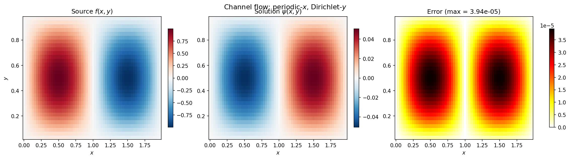
The solver correctly handles the mixed FFT + DST-I combination. The error is at machine precision because the source term is a single eigenmode of the operator.

2. Heated Plate: Dirichlet-x, Neumann-y¶

A rectangular plate with:

• $x$: prescribed temperature on the left and right walls ($\psi = 0$, Dirichlet)
• $y$: insulated top and bottom edges ($\partial\psi/\partial n = 0$, Neumann)

We solve $\nabla^2 \psi = f$ where $f$ is a localised heat source.

In [ ]:

Nx, Ny = 48, 48
Lx, Ly = 1.0, 1.0
dx, dy = Lx / (Nx + 1), Ly / (Ny - 1)

# Interior grid (Dirichlet in x), boundary-inclusive grid (Neumann in y)
x = np.linspace(dx, Lx - dx, Nx)
y = np.linspace(0, Ly, Ny)
X, Y = np.meshgrid(x, y)

# Localised heat source: Gaussian bump
x0, y0, sigma = 0.5, 0.5, 0.1
rhs = jnp.array(-np.exp(-((X - x0) ** 2 + (Y - y0) ** 2) / (2 * sigma**2)))

# Solve
psi = solve_helmholtz_2d(rhs, dx, dy, bc_x="dirichlet", bc_y="neumann")
psi_np = np.array(psi)

fig, axes = plt.subplots(1, 2, figsize=(11, 4.5), constrained_layout=True)

im0 = axes[0].pcolormesh(X, Y, np.array(rhs), cmap="RdBu_r", shading="auto")
axes[0].set_title("Heat source $f(x, y)$")
axes[0].set_xlabel("$x$")
axes[0].set_ylabel("$y$")
axes[0].set_aspect("equal")
fig.colorbar(im0, ax=axes[0], shrink=0.8)

im1 = axes[1].pcolormesh(X, Y, psi_np, cmap="RdBu_r", shading="auto")
axes[1].set_title("Temperature $\\psi(x, y)$")
axes[1].set_xlabel("$x$")
axes[1].set_aspect("equal")
fig.colorbar(im1, ax=axes[1], shrink=0.8)

# Annotate BCs
for ax in axes:
    ax.annotate(
        "$\\psi = 0$",
        xy=(0, 0.5),
        fontsize=9,
        ha="center",
        va="center",
        rotation=90,
        color="blue",
        bbox={"boxstyle": "round,pad=0.2", "fc": "lightyellow", "ec": "blue"},
    )
    ax.annotate(
        "$\\psi = 0$",
        xy=(1, 0.5),
        fontsize=9,
        ha="center",
        va="center",
        rotation=90,
        color="blue",
        bbox={"boxstyle": "round,pad=0.2", "fc": "lightyellow", "ec": "blue"},
    )
    ax.annotate(
        "$\\partial\\psi/\\partial n = 0$",
        xy=(0.5, 0),
        fontsize=8,
        ha="center",
        va="bottom",
        color="green",
        bbox={"boxstyle": "round,pad=0.2", "fc": "lightyellow", "ec": "green"},
    )
    ax.annotate(
        "$\\partial\\psi/\\partial n = 0$",
        xy=(0.5, 1),
        fontsize=8,
        ha="center",
        va="top",
        color="green",
        bbox={"boxstyle": "round,pad=0.2", "fc": "lightyellow", "ec": "green"},
    )

fig.suptitle(
    "Heated plate: Dirichlet-$x$ (walls), Neumann-$y$ (insulated)", fontsize=13, y=1.02
)
fig.savefig(IMG_DIR / "heated_plate.png", dpi=150, bbox_inches="tight")
plt.close(fig)

Nx, Ny = 48, 48 Lx, Ly = 1.0, 1.0 dx, dy = Lx / (Nx + 1), Ly / (Ny - 1) # Interior grid (Dirichlet in x), boundary-inclusive grid (Neumann in y) x = np.linspace(dx, Lx - dx, Nx) y = np.linspace(0, Ly, Ny) X, Y = np.meshgrid(x, y) # Localised heat source: Gaussian bump x0, y0, sigma = 0.5, 0.5, 0.1 rhs = jnp.array(-np.exp(-((X - x0) ** 2 + (Y - y0) ** 2) / (2 * sigma**2))) # Solve psi = solve_helmholtz_2d(rhs, dx, dy, bc_x="dirichlet", bc_y="neumann") psi_np = np.array(psi) fig, axes = plt.subplots(1, 2, figsize=(11, 4.5), constrained_layout=True) im0 = axes[0].pcolormesh(X, Y, np.array(rhs), cmap="RdBu_r", shading="auto") axes[0].set_title("Heat source $f(x, y)$") axes[0].set_xlabel("$x$") axes[0].set_ylabel("$y$") axes[0].set_aspect("equal") fig.colorbar(im0, ax=axes[0], shrink=0.8) im1 = axes[1].pcolormesh(X, Y, psi_np, cmap="RdBu_r", shading="auto") axes[1].set_title("Temperature $\\psi(x, y)$") axes[1].set_xlabel("$x$") axes[1].set_aspect("equal") fig.colorbar(im1, ax=axes[1], shrink=0.8) # Annotate BCs for ax in axes: ax.annotate( "$\\psi = 0$", xy=(0, 0.5), fontsize=9, ha="center", va="center", rotation=90, color="blue", bbox={"boxstyle": "round,pad=0.2", "fc": "lightyellow", "ec": "blue"}, ) ax.annotate( "$\\psi = 0$", xy=(1, 0.5), fontsize=9, ha="center", va="center", rotation=90, color="blue", bbox={"boxstyle": "round,pad=0.2", "fc": "lightyellow", "ec": "blue"}, ) ax.annotate( "$\\partial\\psi/\\partial n = 0$", xy=(0.5, 0), fontsize=8, ha="center", va="bottom", color="green", bbox={"boxstyle": "round,pad=0.2", "fc": "lightyellow", "ec": "green"}, ) ax.annotate( "$\\partial\\psi/\\partial n = 0$", xy=(0.5, 1), fontsize=8, ha="center", va="top", color="green", bbox={"boxstyle": "round,pad=0.2", "fc": "lightyellow", "ec": "green"}, ) fig.suptitle( "Heated plate: Dirichlet-$x$ (walls), Neumann-$y$ (insulated)", fontsize=13, y=1.02 ) fig.savefig(IMG_DIR / "heated_plate.png", dpi=150, bbox_inches="tight") plt.close(fig)

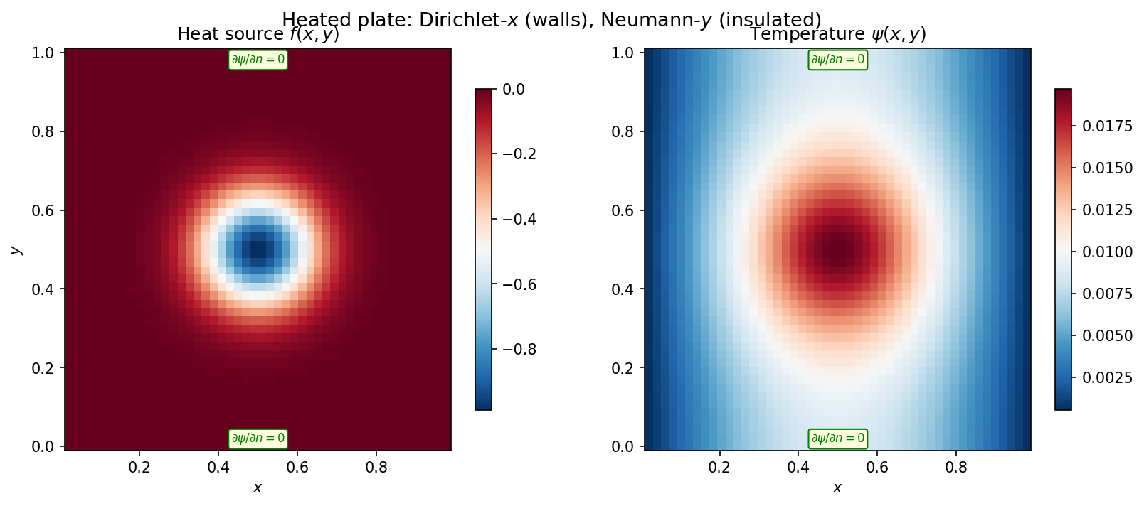
The temperature field shows the expected behaviour:

• The solution vanishes on the left and right walls (Dirichlet).
• The gradient is zero at the top and bottom (Neumann / insulated).
• Heat diffuses outward from the Gaussian source.

3. Half-Pipe: Mixed Left/Right BCs¶

For problems with a symmetry plane, we can use a Dirichlet condition on one side and a Neumann (symmetry) condition on the other. This halves the computational domain.

Here we solve with:

• $x$: Dirichlet-left ($\psi = 0$ at inlet wall) + Neumann-right (symmetry plane)
• $y$: Dirichlet on both walls ($\psi = 0$)

This uses the DST-III transform in $x$ and DST-I in $y$.

In [ ]:

Nx, Ny = 48, 32
Lx, Ly = 1.0, 1.0
dx, dy = Lx / Nx, Ly / (Ny + 1)

# Regular grid for mixed BC in x, interior grid for Dirichlet in y
x = np.arange(Nx) * dx
y = np.linspace(dy, Ly - dy, Ny)
X, Y = np.meshgrid(x, y)

# Uniform source (like pressure-driven flow)
rhs = -jnp.ones((Ny, Nx))

# Solve with mixed left/right BCs on x-axis
psi = solve_helmholtz_2d(
    rhs,
    dx,
    dy,
    bc_x=("dirichlet", "neumann"),  # Dirichlet left, Neumann right
    bc_y="dirichlet",  # Dirichlet both walls
)
psi_np = np.array(psi)

fig, axes = plt.subplots(1, 2, figsize=(12, 4.5), constrained_layout=True)

im0 = axes[0].pcolormesh(X, Y, psi_np, cmap="viridis", shading="auto")
axes[0].set_title("Solution $\\psi(x, y)$")
axes[0].set_xlabel("$x$")
axes[0].set_ylabel("$y$")
axes[0].set_aspect("equal")
fig.colorbar(im0, ax=axes[0], shrink=0.8)

# Cross-sections
axes[1].plot(y, psi_np[:, 0], "o-", ms=3, label=f"$x = {x[0]:.2f}$ (wall)")
axes[1].plot(y, psi_np[:, Nx // 4], "s-", ms=3, label=f"$x = {x[Nx // 4]:.2f}$")
axes[1].plot(y, psi_np[:, Nx // 2], "^-", ms=3, label=f"$x = {x[Nx // 2]:.2f}$")
axes[1].plot(y, psi_np[:, -1], "d-", ms=3, label=f"$x = {x[-1]:.2f}$ (symmetry)")
axes[1].set_xlabel("$y$")
axes[1].set_ylabel("$\\psi$")
axes[1].set_title("Cross-sections at different $x$")
axes[1].legend(fontsize=9)
axes[1].grid(True, alpha=0.3)

# Annotate
axes[0].annotate(
    "$\\psi = 0$\n(wall)",
    xy=(0, 0.5),
    fontsize=9,
    ha="center",
    va="center",
    rotation=90,
    color="blue",
    bbox={"boxstyle": "round,pad=0.2", "fc": "lightyellow", "ec": "blue"},
)
axes[0].annotate(
    "$\\partial\\psi/\\partial n = 0$\n(symmetry)",
    xy=(1, 0.5),
    fontsize=8,
    ha="center",
    va="center",
    rotation=90,
    color="green",
    bbox={"boxstyle": "round,pad=0.2", "fc": "lightyellow", "ec": "green"},
)

fig.suptitle(
    "Half-pipe: Dirichlet-left + Neumann-right ($x$), Dirichlet ($y$)",
    fontsize=13,
    y=1.02,
)
fig.savefig(IMG_DIR / "half_pipe.png", dpi=150, bbox_inches="tight")
plt.close(fig)

Nx, Ny = 48, 32 Lx, Ly = 1.0, 1.0 dx, dy = Lx / Nx, Ly / (Ny + 1) # Regular grid for mixed BC in x, interior grid for Dirichlet in y x = np.arange(Nx) * dx y = np.linspace(dy, Ly - dy, Ny) X, Y = np.meshgrid(x, y) # Uniform source (like pressure-driven flow) rhs = -jnp.ones((Ny, Nx)) # Solve with mixed left/right BCs on x-axis psi = solve_helmholtz_2d( rhs, dx, dy, bc_x=("dirichlet", "neumann"), # Dirichlet left, Neumann right bc_y="dirichlet", # Dirichlet both walls ) psi_np = np.array(psi) fig, axes = plt.subplots(1, 2, figsize=(12, 4.5), constrained_layout=True) im0 = axes[0].pcolormesh(X, Y, psi_np, cmap="viridis", shading="auto") axes[0].set_title("Solution $\\psi(x, y)$") axes[0].set_xlabel("$x$") axes[0].set_ylabel("$y$") axes[0].set_aspect("equal") fig.colorbar(im0, ax=axes[0], shrink=0.8) # Cross-sections axes[1].plot(y, psi_np[:, 0], "o-", ms=3, label=f"$x = {x[0]:.2f}$ (wall)") axes[1].plot(y, psi_np[:, Nx // 4], "s-", ms=3, label=f"$x = {x[Nx // 4]:.2f}$") axes[1].plot(y, psi_np[:, Nx // 2], "^-", ms=3, label=f"$x = {x[Nx // 2]:.2f}$") axes[1].plot(y, psi_np[:, -1], "d-", ms=3, label=f"$x = {x[-1]:.2f}$ (symmetry)") axes[1].set_xlabel("$y$") axes[1].set_ylabel("$\\psi$") axes[1].set_title("Cross-sections at different $x$") axes[1].legend(fontsize=9) axes[1].grid(True, alpha=0.3) # Annotate axes[0].annotate( "$\\psi = 0$\n(wall)", xy=(0, 0.5), fontsize=9, ha="center", va="center", rotation=90, color="blue", bbox={"boxstyle": "round,pad=0.2", "fc": "lightyellow", "ec": "blue"}, ) axes[0].annotate( "$\\partial\\psi/\\partial n = 0$\n(symmetry)", xy=(1, 0.5), fontsize=8, ha="center", va="center", rotation=90, color="green", bbox={"boxstyle": "round,pad=0.2", "fc": "lightyellow", "ec": "green"}, ) fig.suptitle( "Half-pipe: Dirichlet-left + Neumann-right ($x$), Dirichlet ($y$)", fontsize=13, y=1.02, ) fig.savefig(IMG_DIR / "half_pipe.png", dpi=150, bbox_inches="tight") plt.close(fig)

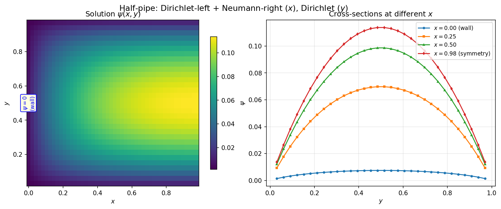
The solution satisfies $\psi = 0$ at the left wall and has zero gradient at the right edge (symmetry plane). The cross-sections show the parabolic profile growing from the wall toward the symmetry plane.

4. Using the Module Class¶

For repeated solves (e.g., in a time-stepping loop), the MixedBCHelmholtzSolver2D class stores the BC configuration and works seamlessly with jax.jit and jax.vmap.

In [ ]:

solver = MixedBCHelmholtzSolver2D(
    dx=dx,
    dy=dy,
    bc_x="periodic",
    bc_y="dirichlet",
)

# Single solve
psi = solver(rhs)

# Batched solve with vmap
rhs_batch = jnp.stack([rhs * (i + 1) for i in range(5)])  # [5, Ny, Nx]
solve_batch = jax.vmap(solver)
psi_batch = solve_batch(rhs_batch)
print(f"Batched solve: {rhs_batch.shape} -> {psi_batch.shape}")

# JIT-compiled solve
solver_jit = jax.jit(solver)
psi_jit = solver_jit(rhs)
print(f"JIT error vs eager: {float(jnp.max(jnp.abs(psi_jit - psi))):.2e}")

solver = MixedBCHelmholtzSolver2D( dx=dx, dy=dy, bc_x="periodic", bc_y="dirichlet", ) # Single solve psi = solver(rhs) # Batched solve with vmap rhs_batch = jnp.stack([rhs * (i + 1) for i in range(5)]) # [5, Ny, Nx] solve_batch = jax.vmap(solver) psi_batch = solve_batch(rhs_batch) print(f"Batched solve: {rhs_batch.shape} -> {psi_batch.shape}") # JIT-compiled solve solver_jit = jax.jit(solver) psi_jit = solver_jit(rhs) print(f"JIT error vs eager: {float(jnp.max(jnp.abs(psi_jit - psi))):.2e}")

Summary¶

Function	Use case
solve_helmholtz_2d(rhs, dx, dy, bc_x=..., bc_y=...)	One-off solves with any BC combination
solve_poisson_2d(rhs, dx, dy, bc_x=..., bc_y=...)	Convenience wrapper with lambda_=0
MixedBCHelmholtzSolver2D(dx, dy, bc_x=..., bc_y=...)	Repeated solves, JIT/vmap friendly

Supported boundary conditions per axis:

BC spec	Transform	Description
"periodic"	FFT	Periodic domain
"dirichlet"	DST-I	$\psi = 0$ on both sides, regular grid
"dirichlet_stag"	DST-II	$\psi = 0$ on both sides, staggered grid
"neumann"	DCT-I	$\partial\psi/\partial n = 0$ on both sides, regular grid
"neumann_stag"	DCT-II	$\partial\psi/\partial n = 0$ on both sides, staggered grid
("dirichlet", "neumann")	DST-III	Dirichlet left + Neumann right, regular
("neumann", "dirichlet")	DCT-III	Neumann left + Dirichlet right, regular
("dirichlet_stag", "neumann_stag")	DST-IV	Dirichlet left + Neumann right, staggered
("neumann_stag", "dirichlet_stag")	DCT-IV	Neumann left + Dirichlet right, staggered

JIT tip: When using the functional API with jax.jit, mark BCs as static:

solve_jit = jax.jit(solve_helmholtz_2d, static_argnames=("bc_x", "bc_y"))