Pseudo-Spectral vs Finite-Difference Eigenvalues¶

SpectralDiffX provides two families of eigenvalues for its spectral elliptic solvers:

Type	Parameter	Formula (Dirichlet)	Accuracy	Use case
FD2	`approximation="fd2"`	$-\frac{4}{\Delta x^2}\sin^2\!\bigl(\frac{\pi(k+1)}{2(N+1)}\bigr)$	$O(h^2)$	Finite-difference / finite-volume codes
Spectral	`approximation="spectral"`	$-\bigl(\frac{\pi(k+1)}{L}\bigr)^2$	Spectral	Pseudo-spectral methods, smooth solutions

The FD2 eigenvalues are the exact inverse of the 3-point finite-difference Laplacian stencil. The pseudo-spectral (PS) eigenvalues are the eigenvalues of the continuous Laplacian $\partial^2/\partial x^2$. They agree for low wavenumbers but diverge near the Nyquist frequency.

This notebook visualises the differences and demonstrates when each matters.

In [ ]:

Copied!





from pathlib import Path

import jax
import jax.numpy as jnp
import matplotlib
import matplotlib.pyplot as plt
import numpy as np

matplotlib.use("Agg")
jax.config.update("jax_enable_x64", True)

from spectraldiffx import (
    dct1_eigenvalues,
    dct1_eigenvalues_ps,
    dct2_eigenvalues,
    dct2_eigenvalues_ps,
    dst1_eigenvalues,
    dst1_eigenvalues_ps,
    dst2_eigenvalues,
    dst2_eigenvalues_ps,
    fft_eigenvalues,
    fft_eigenvalues_ps,
    solve_helmholtz_dst1_1d,
    solve_helmholtz_dst2_1d,
    solve_helmholtz_fft_1d,
)

IMG_DIR = (
    Path(__file__).resolve().parent.parent / "docs" / "images" / "ps_vs_fd2_eigenvalues"
)
IMG_DIR.mkdir(parents=True, exist_ok=True)
from pathlib import Path

import jax
import jax.numpy as jnp
import matplotlib
import matplotlib.pyplot as plt
import numpy as np

matplotlib.use("Agg")
jax.config.update("jax_enable_x64", True)

from spectraldiffx import (
    dct1_eigenvalues,
    dct1_eigenvalues_ps,
    dct2_eigenvalues,
    dct2_eigenvalues_ps,
    dst1_eigenvalues,
    dst1_eigenvalues_ps,
    dst2_eigenvalues,
    dst2_eigenvalues_ps,
    fft_eigenvalues,
    fft_eigenvalues_ps,
    solve_helmholtz_dst1_1d,
    solve_helmholtz_dst2_1d,
    solve_helmholtz_fft_1d,
)

IMG_DIR = (
    Path(__file__).resolve().parent.parent / "docs" / "images" / "ps_vs_fd2_eigenvalues"
)
IMG_DIR.mkdir(parents=True, exist_ok=True)

1. Eigenvalue Curves¶

For a fixed grid with $N = 32$ points, we plot $|\lambda_k|$ for both FD2 and PS eigenvalues across all five same-BC types. The key observation: they agree at low $k$ and diverge at high $k$.

In [ ]:

Copied!





N = 32
dx = 1.0
k = np.arange(N)

configs = [
    ("DST-I (Dirichlet, regular)", dst1_eigenvalues, dst1_eigenvalues_ps, (N + 1) * dx),
    ("DST-II (Dirichlet, staggered)", dst2_eigenvalues, dst2_eigenvalues_ps, N * dx),
    ("DCT-I (Neumann, regular)", dct1_eigenvalues, dct1_eigenvalues_ps, (N - 1) * dx),
    ("DCT-II (Neumann, staggered)", dct2_eigenvalues, dct2_eigenvalues_ps, N * dx),
    ("FFT (periodic)", fft_eigenvalues, fft_eigenvalues_ps, N * dx),
]

fig, axes = plt.subplots(1, 5, figsize=(18, 3.5), constrained_layout=True)

for ax, (title, fd2_fn, ps_fn, L) in zip(axes, configs, strict=False):
    fd2 = np.abs(np.array(fd2_fn(N, dx)))
    ps = np.abs(np.array(ps_fn(N, L)))

    ax.plot(k, fd2, "o-", ms=3, lw=1.2, label="FD2", color="#2196F3")
    ax.plot(k, ps, "s--", ms=3, lw=1.2, label="PS", color="#F44336")
    ax.set_title(title, fontsize=9)
    ax.set_xlabel("Mode $k$", fontsize=9)
    ax.tick_params(labelsize=8)
    if ax == axes[0]:
        ax.set_ylabel("$|\\lambda_k|$", fontsize=10)
    ax.legend(fontsize=8)

fig.suptitle(
    "FD2 vs PS eigenvalues ($N = 32$): agree at low $k$, diverge near Nyquist",
    fontsize=11,
    y=1.02,
)
fig.savefig(IMG_DIR / "eigenvalue_curves.png", dpi=150, bbox_inches="tight")
plt.close(fig)
N = 32
dx = 1.0
k = np.arange(N)

configs = [
    ("DST-I (Dirichlet, regular)", dst1_eigenvalues, dst1_eigenvalues_ps, (N + 1) * dx),
    ("DST-II (Dirichlet, staggered)", dst2_eigenvalues, dst2_eigenvalues_ps, N * dx),
    ("DCT-I (Neumann, regular)", dct1_eigenvalues, dct1_eigenvalues_ps, (N - 1) * dx),
    ("DCT-II (Neumann, staggered)", dct2_eigenvalues, dct2_eigenvalues_ps, N * dx),
    ("FFT (periodic)", fft_eigenvalues, fft_eigenvalues_ps, N * dx),
]

fig, axes = plt.subplots(1, 5, figsize=(18, 3.5), constrained_layout=True)

for ax, (title, fd2_fn, ps_fn, L) in zip(axes, configs, strict=False):
    fd2 = np.abs(np.array(fd2_fn(N, dx)))
    ps = np.abs(np.array(ps_fn(N, L)))

    ax.plot(k, fd2, "o-", ms=3, lw=1.2, label="FD2", color="#2196F3")
    ax.plot(k, ps, "s--", ms=3, lw=1.2, label="PS", color="#F44336")
    ax.set_title(title, fontsize=9)
    ax.set_xlabel("Mode $k$", fontsize=9)
    ax.tick_params(labelsize=8)
    if ax == axes[0]:
        ax.set_ylabel("$|\\lambda_k|$", fontsize=10)
    ax.legend(fontsize=8)

fig.suptitle(
    "FD2 vs PS eigenvalues ($N = 32$): agree at low $k$, diverge near Nyquist",
    fontsize=11,
    y=1.02,
)
fig.savefig(IMG_DIR / "eigenvalue_curves.png", dpi=150, bbox_inches="tight")
plt.close(fig)

FD2 vs PS eigenvalue curves for all five BC types

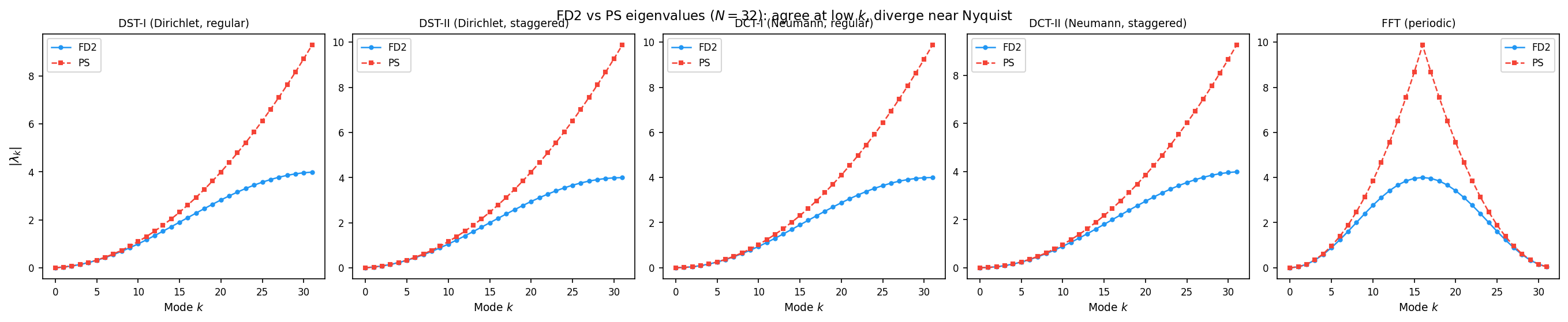
At low wavenumbers ($k \ll N$), the small-angle approximation $\sin(\theta) \approx \theta$ makes the FD2 eigenvalues match the PS ones. Near Nyquist ($k \approx N/2$), the FD2 eigenvalues plateau at $4/\Delta x^2$ while the PS eigenvalues keep growing as $k^2$.

2. Relative Difference¶

The relative error $|\lambda_k^{\text{FD2}} - \lambda_k^{\text{PS}}| / |\lambda_k^{\text{PS}}|$ quantifies when the two families diverge.

In [ ]:

Copied!





fig, ax = plt.subplots(figsize=(7, 4), constrained_layout=True)

colours = ["#2196F3", "#4CAF50", "#FF9800", "#9C27B0", "#F44336"]

for (title, fd2_fn, ps_fn, L), colour in zip(configs, colours, strict=False):
    fd2 = np.array(fd2_fn(N, dx))
    ps = np.array(ps_fn(N, L))
    # Skip k=0 where both may be zero (Neumann/periodic null mode)
    mask = np.abs(ps) > 1e-14
    ps_safe = np.where(mask, np.abs(ps), 1.0)
    rel_err = np.where(mask, np.abs(fd2 - ps) / ps_safe, 0.0)
    ax.semilogy(k, rel_err, "o-", ms=3, lw=1.2, label=title, color=colour)

ax.set_xlabel("Mode $k$", fontsize=10)
ax.set_ylabel("Relative difference", fontsize=10)
ax.set_title("FD2 vs PS relative difference ($N = 32$)")
ax.legend(fontsize=8, loc="upper left")
ax.set_ylim(1e-8, 10)
ax.grid(True, alpha=0.3)
fig.savefig(IMG_DIR / "relative_difference.png", dpi=150, bbox_inches="tight")
plt.close(fig)
fig, ax = plt.subplots(figsize=(7, 4), constrained_layout=True)

colours = ["#2196F3", "#4CAF50", "#FF9800", "#9C27B0", "#F44336"]

for (title, fd2_fn, ps_fn, L), colour in zip(configs, colours, strict=False):
    fd2 = np.array(fd2_fn(N, dx))
    ps = np.array(ps_fn(N, L))
    # Skip k=0 where both may be zero (Neumann/periodic null mode)
    mask = np.abs(ps) > 1e-14
    ps_safe = np.where(mask, np.abs(ps), 1.0)
    rel_err = np.where(mask, np.abs(fd2 - ps) / ps_safe, 0.0)
    ax.semilogy(k, rel_err, "o-", ms=3, lw=1.2, label=title, color=colour)

ax.set_xlabel("Mode $k$", fontsize=10)
ax.set_ylabel("Relative difference", fontsize=10)
ax.set_title("FD2 vs PS relative difference ($N = 32$)")
ax.legend(fontsize=8, loc="upper left")
ax.set_ylim(1e-8, 10)
ax.grid(True, alpha=0.3)
fig.savefig(IMG_DIR / "relative_difference.png", dpi=150, bbox_inches="tight")
plt.close(fig)

Relative difference between FD2 and PS eigenvalues

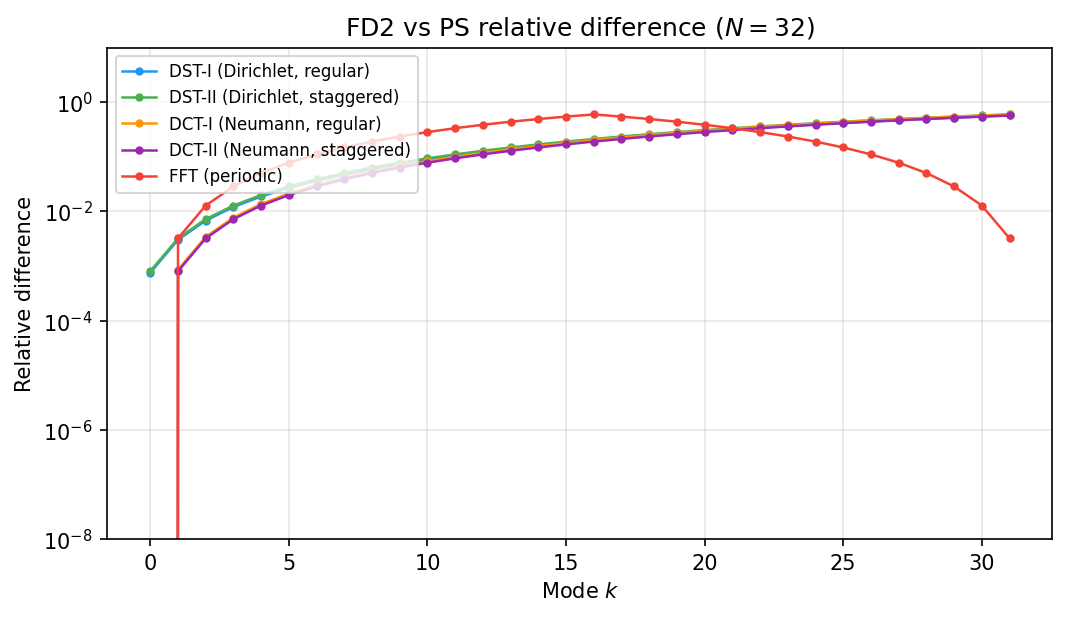
For the first few modes the difference is $< 10^{-3}$. By mode $k = N/2$ (Nyquist), the relative difference exceeds 20%. This means FD2 and PS solvers give essentially the same answer for well-resolved, smooth solutions — the difference only matters at under-resolved scales.

3. Convergence: Spectral vs Second-Order¶

The real payoff of PS eigenvalues is spectral convergence: for smooth test functions, the error drops exponentially with $N$. FD2 eigenvalues give $O(h^2)$ convergence regardless of smoothness.

We solve $\psi''(x) = f(x)$ on $[0, 1]$ with Dirichlet BCs, where $\psi(x) = \sin(4\pi x)$ so that $f(x) = -(4\pi)^2 \sin(4\pi x)$.

In [ ]:

Copied!





resolutions = [8, 12, 16, 24, 32, 48, 64, 96, 128]
errors_fd2_dst1 = []
errors_ps_dst1 = []
errors_fd2_dst2 = []
errors_ps_dst2 = []

for N in resolutions:
    # DST-I: regular grid, L = (N+1)*dx
    dx = 1.0 / (N + 1)
    x = jnp.linspace(dx, 1.0 - dx, N)
    psi_exact = jnp.sin(4 * jnp.pi * x)
    rhs = -((4 * jnp.pi) ** 2) * psi_exact

    psi_fd2 = solve_helmholtz_dst1_1d(rhs, dx, approximation="fd2")
    psi_ps = solve_helmholtz_dst1_1d(rhs, dx, approximation="spectral")
    errors_fd2_dst1.append(float(jnp.max(jnp.abs(psi_fd2 - psi_exact))))
    errors_ps_dst1.append(float(jnp.max(jnp.abs(psi_ps - psi_exact))))

    # DST-II: staggered grid, L = N*dx
    dx2 = 1.0 / N
    x2 = (jnp.arange(N) + 0.5) * dx2
    psi_exact2 = jnp.sin(4 * jnp.pi * x2)
    rhs2 = -((4 * jnp.pi) ** 2) * psi_exact2

    psi_fd2_2 = solve_helmholtz_dst2_1d(rhs2, dx2, approximation="fd2")
    psi_ps_2 = solve_helmholtz_dst2_1d(rhs2, dx2, approximation="spectral")
    errors_fd2_dst2.append(float(jnp.max(jnp.abs(psi_fd2_2 - psi_exact2))))
    errors_ps_dst2.append(float(jnp.max(jnp.abs(psi_ps_2 - psi_exact2))))

N_arr = np.array(resolutions)

fig, axes = plt.subplots(1, 2, figsize=(12, 5), constrained_layout=True)

# DST-I panel
ax = axes[0]
ax.loglog(N_arr, errors_fd2_dst1, "o-", lw=2, ms=5, label="FD2", color="#2196F3")
ax.loglog(
    N_arr, errors_ps_dst1, "s-", lw=2, ms=5, label="PS (spectral)", color="#F44336"
)
# Reference O(h^2) line
ref = errors_fd2_dst1[0] * (N_arr[0] / N_arr) ** 2
ax.loglog(N_arr, ref, "k--", lw=1, alpha=0.5, label="$O(N^{-2})$ reference")
ax.set_xlabel("$N$ (grid points)", fontsize=11)
ax.set_ylabel("Max absolute error", fontsize=11)
ax.set_title("DST-I (Dirichlet, regular grid)")
ax.legend(fontsize=9)
ax.grid(True, alpha=0.3, which="both")
ax.set_ylim(1e-16, 1)

# DST-II panel
ax = axes[1]
ax.loglog(N_arr, errors_fd2_dst2, "o-", lw=2, ms=5, label="FD2", color="#2196F3")
ax.loglog(
    N_arr, errors_ps_dst2, "s-", lw=2, ms=5, label="PS (spectral)", color="#F44336"
)
ref2 = errors_fd2_dst2[0] * (N_arr[0] / N_arr) ** 2
ax.loglog(N_arr, ref2, "k--", lw=1, alpha=0.5, label="$O(N^{-2})$ reference")
ax.set_xlabel("$N$ (grid points)", fontsize=11)
ax.set_title("DST-II (Dirichlet, staggered grid)")
ax.legend(fontsize=9)
ax.grid(True, alpha=0.3, which="both")
ax.set_ylim(1e-16, 1)

fig.suptitle(
    "Convergence: $\\psi(x) = \\sin(4\\pi x)$, Dirichlet BCs",
    fontsize=12,
    y=1.02,
)
fig.savefig(IMG_DIR / "convergence_dirichlet.png", dpi=150, bbox_inches="tight")
plt.close(fig)
resolutions = [8, 12, 16, 24, 32, 48, 64, 96, 128]
errors_fd2_dst1 = []
errors_ps_dst1 = []
errors_fd2_dst2 = []
errors_ps_dst2 = []

for N in resolutions:
    # DST-I: regular grid, L = (N+1)*dx
    dx = 1.0 / (N + 1)
    x = jnp.linspace(dx, 1.0 - dx, N)
    psi_exact = jnp.sin(4 * jnp.pi * x)
    rhs = -((4 * jnp.pi) ** 2) * psi_exact

    psi_fd2 = solve_helmholtz_dst1_1d(rhs, dx, approximation="fd2")
    psi_ps = solve_helmholtz_dst1_1d(rhs, dx, approximation="spectral")
    errors_fd2_dst1.append(float(jnp.max(jnp.abs(psi_fd2 - psi_exact))))
    errors_ps_dst1.append(float(jnp.max(jnp.abs(psi_ps - psi_exact))))

    # DST-II: staggered grid, L = N*dx
    dx2 = 1.0 / N
    x2 = (jnp.arange(N) + 0.5) * dx2
    psi_exact2 = jnp.sin(4 * jnp.pi * x2)
    rhs2 = -((4 * jnp.pi) ** 2) * psi_exact2

    psi_fd2_2 = solve_helmholtz_dst2_1d(rhs2, dx2, approximation="fd2")
    psi_ps_2 = solve_helmholtz_dst2_1d(rhs2, dx2, approximation="spectral")
    errors_fd2_dst2.append(float(jnp.max(jnp.abs(psi_fd2_2 - psi_exact2))))
    errors_ps_dst2.append(float(jnp.max(jnp.abs(psi_ps_2 - psi_exact2))))

N_arr = np.array(resolutions)

fig, axes = plt.subplots(1, 2, figsize=(12, 5), constrained_layout=True)

# DST-I panel
ax = axes[0]
ax.loglog(N_arr, errors_fd2_dst1, "o-", lw=2, ms=5, label="FD2", color="#2196F3")
ax.loglog(
    N_arr, errors_ps_dst1, "s-", lw=2, ms=5, label="PS (spectral)", color="#F44336"
)
# Reference O(h^2) line
ref = errors_fd2_dst1[0] * (N_arr[0] / N_arr) ** 2
ax.loglog(N_arr, ref, "k--", lw=1, alpha=0.5, label="$O(N^{-2})$ reference")
ax.set_xlabel("$N$ (grid points)", fontsize=11)
ax.set_ylabel("Max absolute error", fontsize=11)
ax.set_title("DST-I (Dirichlet, regular grid)")
ax.legend(fontsize=9)
ax.grid(True, alpha=0.3, which="both")
ax.set_ylim(1e-16, 1)

# DST-II panel
ax = axes[1]
ax.loglog(N_arr, errors_fd2_dst2, "o-", lw=2, ms=5, label="FD2", color="#2196F3")
ax.loglog(
    N_arr, errors_ps_dst2, "s-", lw=2, ms=5, label="PS (spectral)", color="#F44336"
)
ref2 = errors_fd2_dst2[0] * (N_arr[0] / N_arr) ** 2
ax.loglog(N_arr, ref2, "k--", lw=1, alpha=0.5, label="$O(N^{-2})$ reference")
ax.set_xlabel("$N$ (grid points)", fontsize=11)
ax.set_title("DST-II (Dirichlet, staggered grid)")
ax.legend(fontsize=9)
ax.grid(True, alpha=0.3, which="both")
ax.set_ylim(1e-16, 1)

fig.suptitle(
    "Convergence: $\\psi(x) = \\sin(4\\pi x)$, Dirichlet BCs",
    fontsize=12,
    y=1.02,
)
fig.savefig(IMG_DIR / "convergence_dirichlet.png", dpi=150, bbox_inches="tight")
plt.close(fig)

Convergence comparison for Dirichlet solvers

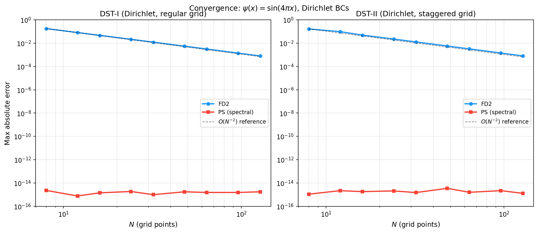
FD2 (blue circles) converges at exactly $O(N^{-2})$ — the dashed reference line confirms second-order. PS (red squares) reaches machine precision ($\sim 10^{-14}$) by $N \approx 32$ for this smooth test function.

The takeaway: if your solution is smooth and you want maximum accuracy per grid point, use approximation="spectral". If you're inverting a finite-difference Laplacian (e.g., in a CFD code), stick with "fd2".

4. Periodic Domain: FFT Convergence¶

The same comparison for periodic BCs.

In [ ]:

Copied!





errors_fd2_fft = []
errors_ps_fft = []

for N in resolutions:
    dx = 1.0 / N
    x = jnp.arange(N) * dx
    psi_exact = jnp.sin(4 * jnp.pi * x)
    rhs = -((4 * jnp.pi) ** 2) * psi_exact

    psi_fd2 = solve_helmholtz_fft_1d(rhs, dx, approximation="fd2")
    psi_ps = solve_helmholtz_fft_1d(rhs, dx, approximation="spectral")
    errors_fd2_fft.append(float(jnp.max(jnp.abs(psi_fd2 - psi_exact))))
    errors_ps_fft.append(float(jnp.max(jnp.abs(psi_ps - psi_exact))))

fig, ax = plt.subplots(figsize=(7, 5), constrained_layout=True)
ax.loglog(N_arr, errors_fd2_fft, "o-", lw=2, ms=5, label="FD2", color="#2196F3")
ax.loglog(
    N_arr, errors_ps_fft, "s-", lw=2, ms=5, label="PS (spectral)", color="#F44336"
)
ref = errors_fd2_fft[0] * (N_arr[0] / N_arr) ** 2
ax.loglog(N_arr, ref, "k--", lw=1, alpha=0.5, label="$O(N^{-2})$ reference")
ax.set_xlabel("$N$ (grid points)", fontsize=11)
ax.set_ylabel("Max absolute error", fontsize=11)
ax.set_title("FFT Periodic: $\\psi(x) = \\sin(4\\pi x)$")
ax.legend(fontsize=10)
ax.grid(True, alpha=0.3, which="both")
ax.set_ylim(1e-16, 1)
fig.savefig(IMG_DIR / "convergence_periodic.png", dpi=150, bbox_inches="tight")
plt.close(fig)
errors_fd2_fft = []
errors_ps_fft = []

for N in resolutions:
    dx = 1.0 / N
    x = jnp.arange(N) * dx
    psi_exact = jnp.sin(4 * jnp.pi * x)
    rhs = -((4 * jnp.pi) ** 2) * psi_exact

    psi_fd2 = solve_helmholtz_fft_1d(rhs, dx, approximation="fd2")
    psi_ps = solve_helmholtz_fft_1d(rhs, dx, approximation="spectral")
    errors_fd2_fft.append(float(jnp.max(jnp.abs(psi_fd2 - psi_exact))))
    errors_ps_fft.append(float(jnp.max(jnp.abs(psi_ps - psi_exact))))

fig, ax = plt.subplots(figsize=(7, 5), constrained_layout=True)
ax.loglog(N_arr, errors_fd2_fft, "o-", lw=2, ms=5, label="FD2", color="#2196F3")
ax.loglog(
    N_arr, errors_ps_fft, "s-", lw=2, ms=5, label="PS (spectral)", color="#F44336"
)
ref = errors_fd2_fft[0] * (N_arr[0] / N_arr) ** 2
ax.loglog(N_arr, ref, "k--", lw=1, alpha=0.5, label="$O(N^{-2})$ reference")
ax.set_xlabel("$N$ (grid points)", fontsize=11)
ax.set_ylabel("Max absolute error", fontsize=11)
ax.set_title("FFT Periodic: $\\psi(x) = \\sin(4\\pi x)$")
ax.legend(fontsize=10)
ax.grid(True, alpha=0.3, which="both")
ax.set_ylim(1e-16, 1)
fig.savefig(IMG_DIR / "convergence_periodic.png", dpi=150, bbox_inches="tight")
plt.close(fig)

Convergence comparison for FFT periodic solver

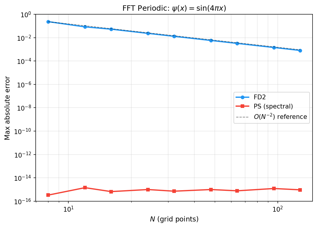
Same story: PS eigenvalues give spectral convergence while FD2 gives $O(h^2)$. For the periodic case, SpectralHelmholtzSolver1D from Layer 1 already uses continuous wavenumbers (equivalent to PS), so approximation="spectral" in the Layer 0 solve_helmholtz_fft_1d now gives the same behaviour.

5. Solution Comparison at Low Resolution¶

At coarse resolution ($N = 16$), the difference between FD2 and PS is visible in the solution itself. Here we solve the same Dirichlet problem and overlay both solutions against the exact answer.

In [ ]:

Copied!





N = 16
dx = 1.0 / (N + 1)
x = np.array(jnp.linspace(dx, 1.0 - dx, N))
psi_exact = np.array(jnp.sin(4 * jnp.pi * jnp.array(x)))

rhs = jnp.array(
    -((4 * jnp.pi) ** 2) * jnp.sin(4 * jnp.pi * jnp.linspace(dx, 1.0 - dx, N))
)
psi_fd2 = np.array(solve_helmholtz_dst1_1d(rhs, dx, approximation="fd2"))
psi_ps = np.array(solve_helmholtz_dst1_1d(rhs, dx, approximation="spectral"))

fig, axes = plt.subplots(1, 2, figsize=(12, 4.5), constrained_layout=True)

# Solutions
ax = axes[0]
x_fine = np.linspace(0, 1, 500)
ax.plot(x_fine, np.sin(4 * np.pi * x_fine), "k-", lw=1.5, label="Exact", alpha=0.4)
ax.plot(x, psi_fd2, "o-", ms=6, lw=1.5, label="FD2", color="#2196F3")
ax.plot(x, psi_ps, "s--", ms=5, lw=1.5, label="PS", color="#F44336")
ax.set_xlabel("$x$", fontsize=11)
ax.set_ylabel("$\\psi(x)$", fontsize=11)
ax.set_title(f"Solution ($N = {N}$)")
ax.legend(fontsize=9)
ax.grid(True, alpha=0.3)

# Errors
ax = axes[1]
ax.plot(
    x,
    np.abs(psi_fd2 - psi_exact),
    "o-",
    ms=5,
    lw=1.5,
    label="FD2 error",
    color="#2196F3",
)
ax.plot(
    x, np.abs(psi_ps - psi_exact), "s-", ms=5, lw=1.5, label="PS error", color="#F44336"
)
ax.set_xlabel("$x$", fontsize=11)
ax.set_ylabel("$|\\psi - \\psi_{\\text{exact}}|$", fontsize=11)
ax.set_title(f"Pointwise error ($N = {N}$)")
ax.set_yscale("log")
ax.legend(fontsize=9)
ax.grid(True, alpha=0.3)

fig.savefig(IMG_DIR / "solution_comparison.png", dpi=150, bbox_inches="tight")
plt.close(fig)
N = 16
dx = 1.0 / (N + 1)
x = np.array(jnp.linspace(dx, 1.0 - dx, N))
psi_exact = np.array(jnp.sin(4 * jnp.pi * jnp.array(x)))

rhs = jnp.array(
    -((4 * jnp.pi) ** 2) * jnp.sin(4 * jnp.pi * jnp.linspace(dx, 1.0 - dx, N))
)
psi_fd2 = np.array(solve_helmholtz_dst1_1d(rhs, dx, approximation="fd2"))
psi_ps = np.array(solve_helmholtz_dst1_1d(rhs, dx, approximation="spectral"))

fig, axes = plt.subplots(1, 2, figsize=(12, 4.5), constrained_layout=True)

# Solutions
ax = axes[0]
x_fine = np.linspace(0, 1, 500)
ax.plot(x_fine, np.sin(4 * np.pi * x_fine), "k-", lw=1.5, label="Exact", alpha=0.4)
ax.plot(x, psi_fd2, "o-", ms=6, lw=1.5, label="FD2", color="#2196F3")
ax.plot(x, psi_ps, "s--", ms=5, lw=1.5, label="PS", color="#F44336")
ax.set_xlabel("$x$", fontsize=11)
ax.set_ylabel("$\\psi(x)$", fontsize=11)
ax.set_title(f"Solution ($N = {N}$)")
ax.legend(fontsize=9)
ax.grid(True, alpha=0.3)

# Errors
ax = axes[1]
ax.plot(
    x,
    np.abs(psi_fd2 - psi_exact),
    "o-",
    ms=5,
    lw=1.5,
    label="FD2 error",
    color="#2196F3",
)
ax.plot(
    x, np.abs(psi_ps - psi_exact), "s-", ms=5, lw=1.5, label="PS error", color="#F44336"
)
ax.set_xlabel("$x$", fontsize=11)
ax.set_ylabel("$|\\psi - \\psi_{\\text{exact}}|$", fontsize=11)
ax.set_title(f"Pointwise error ($N = {N}$)")
ax.set_yscale("log")
ax.legend(fontsize=9)
ax.grid(True, alpha=0.3)

fig.savefig(IMG_DIR / "solution_comparison.png", dpi=150, bbox_inches="tight")
plt.close(fig)

Solution and error comparison at N=16

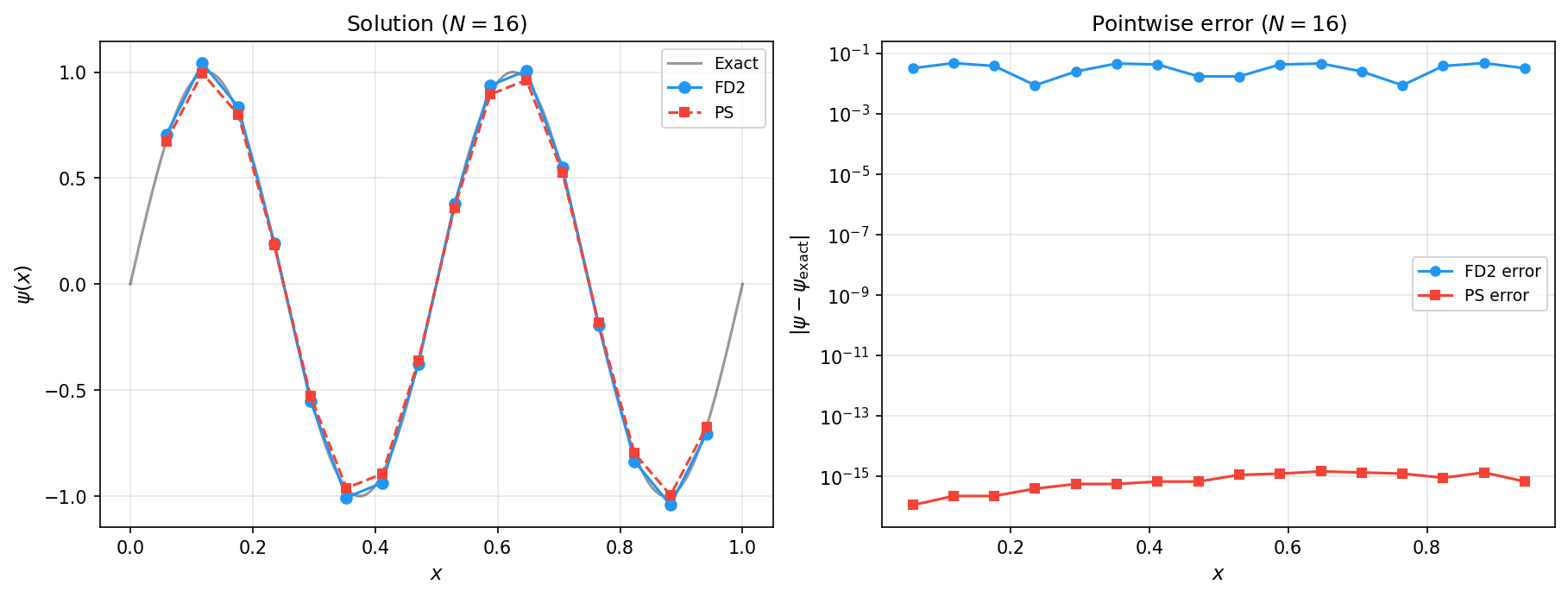
At $N = 16$, FD2 shows visible deviation from the exact solution (left panel), with pointwise errors of $O(10^{-2})$ (right panel). The PS solution is accurate to $\sim 10^{-13}$ — essentially machine precision.

Summary¶

	FD2 (`"fd2"`)	PS (`"spectral"`)
Formula	$-4/\Delta x^2 \cdot \sin^2(\ldots)$	$-(\pi k / L)^2$
Convergence	$O(h^2)$	Spectral (exponential)
Exact inverse of	3-point FD stencil	Continuous Laplacian
Best for	FD/FV codes, operator splitting	Pseudo-spectral methods
Default	Yes	No

# Use FD2 (default) for finite-difference codes
psi = solve_helmholtz_dst(rhs, dx, dy)

# Use spectral for maximum accuracy with smooth data
psi = solve_helmholtz_dst(rhs, dx, dy, approximation="spectral")