Modern 4DVar

State Estimation - Strong Constrained 4DVar

How to estimate the state using a dynamical ODE

CNRS

MEOM

import os, sys

jaxsw_path = "/Users/eman/code_projects/jaxsw"
sys.path.append(jaxsw_path)

import autoroot  # noqa: F401, I001
import jax
import jax.numpy as jnp
import jax.random as jrandom
import numpy as np
import matplotlib.pyplot as plt
import seaborn as sns
import diffrax as dfx
import equinox as eqx
import xarray as xr
import functools as ft

from jaxsw import L63State, Lorenz63, rhs_lorenz_63

jax.config.update("jax_enable_x64", True)

sns.reset_defaults()
sns.set_context(context="talk", font_scale=0.7)

%matplotlib inline
%load_ext autoreload
%autoreload 2

Lorenz 63¶

Equation of Motion
Observation Operator
Integrate

Equation of Motion¶

\begin{aligned} \frac{dx}{dt} &= \sigma (y - x) \\ \frac{dy}{dt} &= x (\rho - z) - y \\ \frac{dz}{dt} &= xy - \beta z \end{aligned}

(1)

where $(\sigma,\rho,\beta)$ are hyperparameters.

Simulation¶

ds_sol = xr.open_dataset("./data/sim_l63.nc")
ds_sol

Inverse Problem¶

realization = 100

ds_trajectory = ds_sol.sel(realization=realization)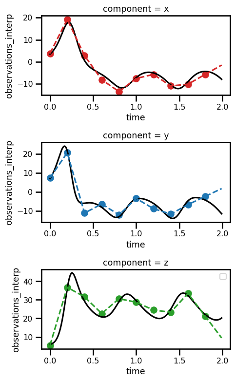
ds_trajectory

fig, ax = plt.subplots(nrows=3, figsize=(5, 8))


ds_trajectory.simulation.sel(component="x").plot(ax=ax[0], color="black")
ds_trajectory.simulation.sel(component="y").plot(ax=ax[1], color="black")
ds_trajectory.simulation.sel(component="z").plot(ax=ax[2], color="black")

ds_trajectory.observations_noise.sel(component="x").plot.scatter(
    ax=ax[0], color="tab:red"
)
ds_trajectory.observations_noise.sel(component="y").plot.scatter(
    ax=ax[1], color="tab:blue"
)
ds_trajectory.observations_noise.sel(component="z").plot.scatter(
    ax=ax[2], color="tab:green"
)

ds_trajectory.observations_interp.sel(component="x").plot(
    ax=ax[0], color="tab:red", linestyle="--"
)
ds_trajectory.observations_interp.sel(component="y").plot(
    ax=ax[1], color="tab:blue", linestyle="--"
)
ds_trajectory.observations_interp.sel(component="z").plot(
    ax=ax[2], color="tab:green", linestyle="--"
)

# ax.set_xlabel("Time")
# ax.set_ylabel("Values")
# ax.set_title(f"Trajectory")


plt.legend()
plt.tight_layout()
plt.show()

No artists with labels found to put in legend.  Note that artists whose label start with an underscore are ignored when legend() is called with no argument.

Data¶

For this problem we need the following variables

True State: $\boldsymbol{u}$

Time Steps: $\boldsymbol{\Tau}$

Observations: $\boldsymbol{y}$

Initial State: $\boldsymbol{u}^{(k)}$

Mask: $\boldsymbol{m}$

# Ground Truth
x_state = jnp.asarray(ds_trajectory.simulation.values).T.astype(jnp.float64)
ts_state = jnp.asarray(ds_trajectory.time.values).astype(jnp.float64)
# Observations
y_gt = jnp.asarray(ds_trajectory.observations_noise.values).T.astype(jnp.float64)
# Mask
y_mask = 1.0 - (
    jnp.isnan(jnp.asarray(ds_trajectory.observations_noise.values))
    .astype(jnp.float32)
    .T.astype(jnp.float64)
)
# initialization
x_init = jnp.asarray(ds_trajectory.observations_interp.values).T.astype(jnp.float64)

x_state.shape, y_gt.shape, y_mask.shape, x_init.shape

((200, 3), (200, 3), (200, 3), (200, 3))

Dynamical Prior¶

Here, we define our dynamical prior which we plug into this loss function.

\mathbf{R}(\boldsymbol{u};\boldsymbol{\theta}) = \frac{\lambda}{2} ||\boldsymbol{u} - \boldsymbol{\phi}(\boldsymbol{u};\boldsymbol{\theta})||_2^2

(2)

Our dynamical prior in this case is defined by:

\boldsymbol{\phi}(\boldsymbol{u};\boldsymbol{\theta}) \coloneqq \boldsymbol{u}(t_1) = \boldsymbol{u}(t_0) + \int_{t_0}^{t_1} \boldsymbol{F}\left( \boldsymbol{u}(t),\tau;\boldsymbol{\theta}\right)d\tau

(3)

Strong Constrained

The strong-constrained version works by applying the solver directly through the entire trajectory from start to finish. We are sure to output the state during moments of the trajectory to ensure that we can check to ensure that we can check out how well they match the observations. So, the function will look something like:

\left[ \boldsymbol{u}_T, \boldsymbol{u}_{T-\Delta t}, \ldots, \boldsymbol{u}_{\Delta t}, \boldsymbol{u}_0\right] = \text{ODESolve}\left(\boldsymbol{F}, \boldsymbol{u}_0, T, \Delta t, \boldsymbol{\theta}, \right)

(4)

whereby we get a matrix, $\mathbf{U}\in\mathbb{R}^{D_T\times D_u}$ , which contains all of the state vectors for every time step of interest. So our $\boldsymbol{\phi}$ operator will be

\mathbf{U} = \boldsymbol{\phi}(\boldsymbol{u},t;\boldsymbol{\theta})

(5)

and our cost function will be

\mathbf{R}(\boldsymbol{u};\boldsymbol{\theta}) = \frac{\lambda}{2} \sum_{t=0}^T ||\boldsymbol{u}_t - \boldsymbol{\phi}(\boldsymbol{u};\boldsymbol{\theta})_t||_2^2

(6)

from mfourdvar._src.priors.dynamical import DynIncrements, DynTrajectory
from jaxsw import L63State, L63Params

import typing as tp
from jaxtyping import Array, PyTree

class L63Params(eqx.Module):
    sigma: Array = eqx.static_field()
    rho: Array = eqx.static_field()
    beta: Array = eqx.static_field()
    
    def __init__(self, sigma: float=10., rho: float=28., beta: float=2.667):
        self.sigma = jnp.asarray(sigma, dtype=jnp.float64)
        self.rho = jnp.asarray(rho, dtype=jnp.float64)
        self.beta = jnp.asarray(beta, dtype=jnp.float64)

class L63Model(eqx.Module):
    model: PyTree

    def init_state(self, x: PyTree) -> PyTree:
        state = L63State(
            x=jnp.atleast_1d(x[..., 0]), 
            y=jnp.atleast_1d(x[..., 1]), 
            z=jnp.atleast_1d(x[..., 2])
        )
        return state
    
    def __call__(self, t, state, args):
        return self.model.equation_of_motion(t, state, args)

x_init.shape

(200, 3)

# init dynamical system
l63_dyn_model = Lorenz63()

# initialize prior model
prior_model = L63Model(model=l63_dyn_model)


# initialize state
state_init = prior_model.init_state(x_init[0])

# initialize params
params = L63Params(sigma=10., rho=28., beta=2.667)


# output state
state_out = prior_model(0, state_init, params)

# check input and output are the same
assert state_init.x.shape == state_out.x.shape
assert state_init.y.shape == state_out.y.shape
assert state_init.z.shape == state_out.z.shape

x_init[0].dtype, ts_state[1:].dtype

(dtype('float64'), dtype('float64'))

# initialize dynamical prior
prior = DynTrajectory(model=prior_model, params=params)

# forward for prior
out = prior(x=x_init[0] + 5., ts=ts_state[1:])
out.x.shape, out.y.shape, out.z.shape, ts_state.shape

((199, 1), (199, 1), (199, 1), (200,))

Loss Function¶

We already have access to the loss function via this convenient prior class. It automatically implements a simple dynamical loss in terms of MSE.

loss = prior.loss(x_init, ts_state, )
loss

Array(6825.24488202, dtype=float64)

Gradient Function¶

Now, we need to take the derivatives wrt the state. The prior model, the params and the time steps are all going to state constant s

prior = DynTrajectory(model=prior_model)

@ft.partial(jax.value_and_grad)
def loss_function_state(x_init, params):
    return prior.loss(x_init, ts_state, params=params)

loss, grads = loss_function_state(x_init, params)
print(grads.shape)


@eqx.filter_value_and_grad
def loss_function_state(x_init, params):
    return prior.loss(x_init, ts_state, params=params)

loss, grads = loss_function_state(x_init, params)
print(grads.shape)
loss

(200, 3)
(200, 3)

Array(6825.24488202, dtype=float64)

fig, ax = plt.subplots()

ax.plot(ts_state, grads[..., 0].squeeze(), linestyle="-", color="tab:blue")
ax.plot(ts_state, grads[..., 1].squeeze(), linestyle="-", color="tab:orange")
ax.plot(ts_state, grads[..., 2].squeeze(), linestyle="-", color="tab:green")

[<matplotlib.lines.Line2D at 0x298921730>]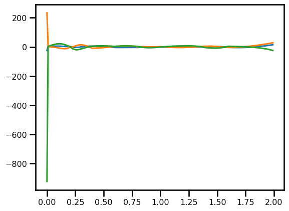

Parameter Gradients¶

@ft.partial(jax.value_and_grad)
def loss_function_params(params, x_init):
    return prior.loss(x_init, ts_state, params=params)

loss, grads = loss_function_params(params, x_init)
print(grads)


@eqx.filter_value_and_grad
def loss_function_params(params, x_init):
    
    return prior.loss(x_init, ts_state, params=params)

loss, grads = loss_function_params(params, x_init)
print(grads)
loss

L63Params(sigma=f64[], rho=f64[], beta=f64[])
L63Params(sigma=f64[], rho=f64[], beta=f64[])

Array(6825.24488202, dtype=float64)

fig, ax = plt.subplots()

ax.plot(ts_state[1:], out.array[..., 0].squeeze(), linestyle="-", color="tab:blue")
ax.plot(ts_state, x_state[..., 0].squeeze(), linestyle="--", color="tab:blue")
ax.scatter(ts_state, y_gt[..., 0], color="tab:blue")
ax.plot(ts_state[1:], out.array[..., 1].squeeze(), linestyle="-", color="tab:orange")
ax.plot(ts_state, x_state[..., 1].squeeze(), linestyle="--", color="tab:orange")
ax.scatter(ts_state, y_gt[..., 1], color="tab:orange")
ax.plot(ts_state[1:], out.array[..., 2].squeeze(), linestyle="-", color="tab:green")
ax.plot(ts_state, x_state[..., 2].squeeze(), linestyle="--", color="tab:green")
ax.scatter(ts_state, y_gt[..., 2],  color="tab:green")

<matplotlib.collections.PathCollection at 0x2989cd550>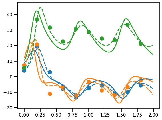

Learning¶

In this instance, we're going to use a simple gradient descent scheme.

\boldsymbol{u}^{(k+1)} = \boldsymbol{u}^{(k)} + \alpha \boldsymbol{\nabla_u}\boldsymbol{J}(\boldsymbol{u};\boldsymbol{\theta})

(7)

where $\alpha$ is the learning rate and $\boldsymbol{\nabla_u}$ is the gradient operator wrt the state, $\boldsymbol{u}$ . We have an optimality condition of the gradient of the variational cost.

\boldsymbol{F_g}(\boldsymbol{u};\boldsymbol{\theta}) = \boldsymbol{\nabla_u}\boldsymbol{J}(\boldsymbol{u};\boldsymbol{\theta})

(8)

Because we are doing gradient descent, we will use a negative learning rate of $\alpha=-0.1$ .

For this first part, we're simply going to use the variational cost as the dynamical prior.

\begin{aligned} \boldsymbol{J}(\boldsymbol{u};\boldsymbol{\theta}) &= \boldsymbol{R}(\boldsymbol{u};\boldsymbol{\theta}) \\ &= \frac{\lambda}{2} \sum_{t=0}^T ||\boldsymbol{u}_t - \boldsymbol{\phi}(\boldsymbol{u}_t;\boldsymbol{\theta})||_2^2 \end{aligned}

(9)

Observation Operator¶

\boldsymbol{L}(\boldsymbol{u};\boldsymbol{\theta}) = \lambda_{obs}|| \boldsymbol{y} - \boldsymbol{H}(\boldsymbol{u};\boldsymbol{\theta})||_2^2

(10)

We can use a simpler loss function which is just a masking operator.

\boldsymbol{L}(\boldsymbol{u};\boldsymbol{\theta}) = \lambda_{obs}|| \boldsymbol{y} - \boldsymbol{u}||_{\Omega_{obs}}^2

(11)

where $\Omega_{obs}$ is the domain of the observation.

from mfourdvar._src.operators.base import ObsOperator

obs_operator = ObsOperator()

obs_operator.loss(x_init, y_gt, y_mask)

Array(0., dtype=float64)

Variational Cost¶

from mfourdvar._src.varcost.dynamical import StrongVarCost

# init dynamical system
l63_dyn_model = Lorenz63()

# initialize prior model
prior_model = L63Model(model=l63_dyn_model)
# initialize params
params = L63Params(sigma=10., rho=28., beta=2.667)
# initialize dynamical prior
prior = DynTrajectory(model=prior_model, params=params)

# initialize observation operator
obs_operator = ObsOperator()

# initialize variational cost function
prior_weight = 1.0
obs_op_weight = 0.1
background_weight = 0.1
varcost_fn = StrongVarCost(
    prior=prior, 
    obs_op=obs_operator, 
    prior_weight=prior_weight, 
    obs_op_weight=obs_op_weight, 
    background_weight=background_weight
)

loss_init, losses_init = varcost_fn.loss(x=x_init[0], ts=ts_state, y=y_gt, mask=y_mask, return_loss=True)
loss_true, losses_true = varcost_fn.loss(x=x_state[0], ts=ts_state, y=y_gt,  mask=y_mask, return_loss=True)

loss_init, losses_init

(Array(13.13013833, dtype=float64),
 {'var_loss': Array(13.13013833, dtype=float64),
  'obs': Array(116.67463353, dtype=float64),
  'bg': Array(14.62674975, dtype=float64)})

print("True State vs True State")
print(losses_true)
print("Init X vs Init State") 
print(losses_init)

True State vs True State
{'var_loss': Array(12.20563867, dtype=float64), 'obs': Array(103.49842271, dtype=float64), 'bg': Array(18.55796399, dtype=float64)}
Init X vs Init State
{'var_loss': Array(13.13013833, dtype=float64), 'obs': Array(116.67463353, dtype=float64), 'bg': Array(14.62674975, dtype=float64)}

Learning¶

@ft.partial(jax.value_and_grad, has_aux=True)
def loss_function_state(x_init):    
    return varcost_fn.loss(x=x_init, ts=ts_state, y=y_gt,  mask=y_mask, return_loss=True)

(loss, _), grads = loss_function_state(x_init[0])
print(grads.shape)

@eqx.filter_value_and_grad(has_aux=True)
def loss_function_state(x_init):    
    return varcost_fn.loss(x=x_init, ts=ts_state, y=y_gt,  mask=y_mask, return_loss=True)

(loss, _), grads = loss_function_state(x_init[0])
print(grads.shape)
loss

(3,)
(3,)

Array(13.13013833, dtype=float64)

from tqdm.autonotebook import trange

losses = dict(prior=[], obs=[], bg=[], var_loss=[])
num_iterations = 100
learning_rate = - 0.2
x0 = x_init.copy()[0]

# loop through learning
with trange(num_iterations) as pbar:
    for i in pbar:

        # get dynamical loss + gradient
        (_, loss), x_grad = loss_function_state(x0)

        losses["var_loss"].append(loss["var_loss"])
        losses["obs"].append(loss["obs"])
        losses["bg"].append(loss["bg"])

        pbar_msg = f"Var Loss: {loss['var_loss']:.2e} | "
        pbar_msg += f"Obs - {loss['obs']:.2e} | "
        pbar_msg += f"BG - {loss['bg']:.2e}"
        pbar.set_description(pbar_msg)

        # clip gradients (prevent explosion)
        x_grad = jnp.clip(x_grad, a_min=-0.5, a_max=0.5)

        # update solution with gradient
        x0 += learning_rate * x_grad

x0, x_init[0], grads

(Array([4.55909722, 5.4635627 , 5.325818  ], dtype=float64),
 Array([3.83415643, 7.27995046, 5.49344943], dtype=float64),
 Array([ 1.6533432 ,  3.49085841, -1.43647224], dtype=float64))

# compute variational cost
loss_init, losses_init = varcost_fn.loss(x=x_init[0], ts=ts_state, y=y_gt, mask=y_mask, return_loss=True)
loss_true, losses_true = varcost_fn.loss(x=x_state[0], ts=ts_state, y=y_gt, mask=y_mask, return_loss=True)
loss_sol_true, losses_sol_true = varcost_fn.loss(x=x0, ts=ts_state, y=y_gt, mask=y_mask, return_loss=True)

print("True State vs True State")
print(losses_true)
print("Init X vs Init State") 
print(losses_init)
print("Sol State vs True State")
print(losses_sol_true)

True State vs True State
{'var_loss': Array(12.20563867, dtype=float64), 'obs': Array(103.49842271, dtype=float64), 'bg': Array(18.55796399, dtype=float64)}
Init X vs Init State
{'var_loss': Array(13.13013833, dtype=float64), 'obs': Array(116.67463353, dtype=float64), 'bg': Array(14.62674975, dtype=float64)}
Sol State vs True State
{'var_loss': Array(10.67219794, dtype=float64), 'obs': Array(105.31606079, dtype=float64), 'bg': Array(1.40591857, dtype=float64)}

fig, ax = plt.subplots()

ax.plot(losses["obs"], label="Observations", linestyle=":")
ax.plot(losses["bg"], label="Background", linestyle=":")
ax.plot(losses["var_loss"], label="Variational", zorder=0)

ax.set(
    yscale="log",
    xscale="log",
    xlabel="Iterations", 
    ylabel="Loss"
)

plt.legend()
plt.show()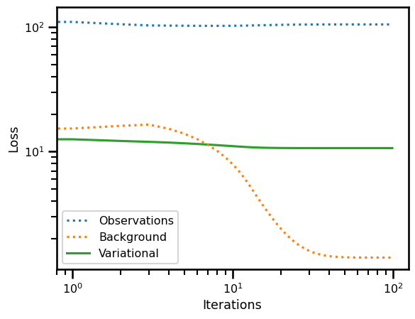

x = prior(x0, ts_state)
x = x.array
x0.shape, x.shape

((3,), (200, 3))

ds_results = xr.Dataset(
    {
        "x": (("time"), x[:, 0].squeeze()),
        "y": (("time"), x[:, 1].squeeze()),
        "z": (("time"), x[:, 2].squeeze()),
    },
    coords={
        "time": (["time"], ts_state.squeeze()),
    },
    attrs={
        "ode": "lorenz_63",
        "sigma": params.sigma,
        "beta": params.beta,
        "rho": params.rho,
    },
)

ds_results = ds_results.to_array(dim="component", name="prediction").to_dataset()
ds_results["state"] = (
    (
        "component",
        "time",
    ),
    x_state.T,
)
ds_results["initialization"] = (
    (
        "component",
        "time",
    ),
    x_init.T,
)
ds_results["observation"] = (
    (
        "component",
        "time",
    ),
    y_gt.T,
)
# ds_results.x_state
ds_results

fig, ax = plt.subplots(nrows=3, figsize=(5, 8))

for axis in range(3):
    ds_results.state.isel(component=axis).plot(
        ax=ax[axis], linestyle="-", color="black", label="True"
    )
    ds_results.prediction.isel(component=axis).plot(
        ax=ax[axis], linestyle="-", color="tab:green", label="Predict"
    )
    ds_results.initialization.isel(component=axis).plot(
        ax=ax[axis], linestyle=":", color="tab:blue", label="Initialization"
    )
    ds_results.observation.isel(component=axis).plot.scatter(
        ax=ax[axis], color="tab:red", label="Observations"
    )
    plt.legend()


# plt.legend()
plt.tight_layout()
plt.show()

No artists with labels found to put in legend.  Note that artists whose label start with an underscore are ignored when legend() is called with no argument.
No artists with labels found to put in legend.  Note that artists whose label start with an underscore are ignored when legend() is called with no argument.

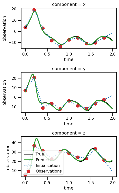
Crazier Initial Condition¶

from tqdm.autonotebook import trange

losses = dict(prior=[], obs=[], bg=[], var_loss=[])
num_iterations = 100
learning_rate = - 0.2
x0 = x_init.copy()[0] + 5.0

# loop through learning
with trange(num_iterations) as pbar:
    for i in pbar:

        # get dynamical loss + gradient
        (_, loss), x_grad = loss_function_state(x0)

        losses["var_loss"].append(loss["var_loss"])
        losses["obs"].append(loss["obs"])
        losses["bg"].append(loss["bg"])

        pbar_msg = f"Var Loss: {loss['var_loss']:.2e} | "
        pbar_msg += f"Obs - {loss['obs']:.2e} | "
        pbar_msg += f"BG - {loss['bg']:.2e}"
        pbar.set_description(pbar_msg)

        # clip gradients (prevent explosion)
        x_grad = jnp.clip(x_grad, a_min=-0.5, a_max=0.5)

        # update solution with gradient
        x0 += learning_rate * x_grad

x_init[0], grads

(Array([3.83415643, 7.27995046, 5.49344943], dtype=float64),
 Array([ 1.6533432 ,  3.49085841, -1.43647224], dtype=float64))

# compute variational cost
loss_init, losses_init = varcost_fn.loss(x=x_init[0] + 5., ts=ts_state, y=y_gt, mask=y_mask, return_loss=True)
loss_true, losses_true = varcost_fn.loss(x=x_state[0], ts=ts_state, y=y_gt, mask=y_mask, return_loss=True)
loss_sol_true, losses_sol_true = varcost_fn.loss(x=x0, ts=ts_state, y=y_gt, mask=y_mask, return_loss=True)

print("True State vs True State")
print(losses_true)
print("Init X vs Init State") 
print(losses_init)
print("Sol State vs True State")
print(losses_sol_true)

True State vs True State
{'var_loss': Array(12.20563867, dtype=float64), 'obs': Array(103.49842271, dtype=float64), 'bg': Array(18.55796399, dtype=float64)}
Init X vs Init State
{'var_loss': Array(72.42176102, dtype=float64), 'obs': Array(709.59086047, dtype=float64), 'bg': Array(14.62674975, dtype=float64)}
Sol State vs True State
{'var_loss': Array(10.67220015, dtype=float64), 'obs': Array(105.30777161, dtype=float64), 'bg': Array(1.41422986, dtype=float64)}

fig, ax = plt.subplots()

ax.plot(losses["obs"], label="Observations", linestyle=":")
ax.plot(losses["bg"], label="Background", linestyle=":")
ax.plot(losses["var_loss"], label="Variational", zorder=0)

ax.set(
    yscale="log",
    xscale="log",
    xlabel="Iterations", 
    ylabel="Loss"
)

plt.legend()
plt.show()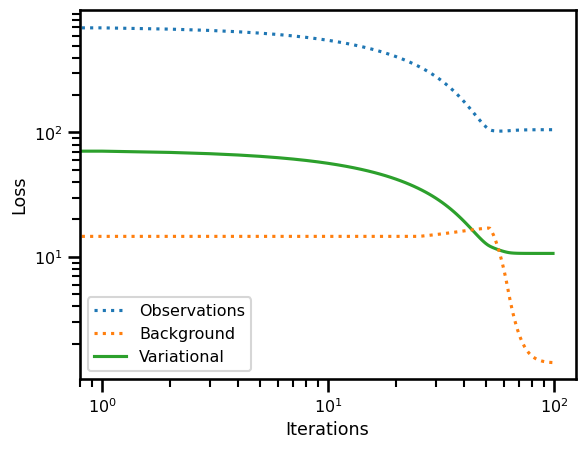

x = prior(x0, ts_state)
x = x.array
x0.shape, x.shape

((3,), (200, 3))

ds_results = xr.Dataset(
    {
        "x": (("time"), x[:, 0].squeeze()),
        "y": (("time"), x[:, 1].squeeze()),
        "z": (("time"), x[:, 2].squeeze()),
    },
    coords={
        "time": (["time"], ts_state.squeeze()),
    },
    attrs={
        "ode": "lorenz_63",
        "sigma": params.sigma,
        "beta": params.beta,
        "rho": params.rho,
    },
)

ds_results = ds_results.to_array(dim="component", name="prediction").to_dataset()
ds_results["state"] = (
    (
        "component",
        "time",
    ),
    x_state.T,
)
ds_results["initialization"] = (
    (
        "component",
        "time",
    ),
    x_init.T,
)
ds_results["observation"] = (
    (
        "component",
        "time",
    ),
    y_gt.T,
)
# ds_results.x_state
ds_results

fig, ax = plt.subplots(nrows=3, figsize=(5, 8))

for axis in range(3):
    ds_results.state.isel(component=axis).plot(
        ax=ax[axis], linestyle="-", color="black", label="True"
    )
    ds_results.prediction.isel(component=axis).plot(
        ax=ax[axis], linestyle="-", color="tab:green", label="Predict"
    )
    ds_results.initialization.isel(component=axis).plot(
        ax=ax[axis], linestyle=":", color="tab:blue", label="Initialization"
    )
    ds_results.observation.isel(component=axis).plot.scatter(
        ax=ax[axis], color="tab:red", label="Observations"
    )
    plt.legend()


# plt.legend()
plt.tight_layout()
plt.show()

No artists with labels found to put in legend.  Note that artists whose label start with an underscore are ignored when legend() is called with no argument.
No artists with labels found to put in legend.  Note that artists whose label start with an underscore are ignored when legend() is called with no argument.