Marginal transforms: ECDF & histograms
The atom of Gaussianization — rank → uniform → normal — and where the empirical CDF breaks
00 — Marginal transforms: ECDF & histograms
Part 0 showed what a density destructor is. Part 1 builds its atom: the per-coordinate map that turns one messy marginal into a standard normal. Every method in this curriculum — RBIG, coupling flows, spline flows — is ultimately a stack of these 1D transforms interleaved with rotations. Get the 1D piece right and the rest is composition (notebook 01 of Part 0).
What you will see
- The probability integral transform and why it Gaussianizes any continuous marginal — if we know .
- Estimating with the empirical CDF and a histogram CDF.
- Glivenko–Cantelli: the ECDF converges uniformly to as .
- The rank → uniform → normal pipeline with
rbigandgauss_flows. - The boundary failure of the ECDF in the tails — the motivation for the smooth estimators (KDE, mixtures, splines) in the rest of Part 1.
import warnings

warnings.filterwarnings("ignore")

import jax
import jax.numpy as jnp
import matplotlib.pyplot as plt
import numpy as np
from scipy import stats

import gauss_flows as gf
import rbig
from _style import GAUSS_KW, style_ax

jax.config.update("jax_enable_x64", True)
rng = np.random.default_rng(10)

# A skewed, strictly-positive marginal to Gaussianize (well away from normal).
x = rng.exponential(1.0, size=(6000, 1))
1. The probability integral transform
The whole idea rests on one classical fact. If a continuous random variable has strictly increasing CDF , then is uniform on (the probability integral transform, PIT). Composing with the standard-normal quantile then sends that uniform to a standard normal:
So in 1D we can Gaussianize exactly — given the true . The catch is that we never know ; we must estimate it from samples. The two simplest estimators are the empirical CDF and the histogram, and seeing how (and where) they fail sets up everything else in Part 1.
2. The empirical CDF and Glivenko–Cantelli
The empirical CDF just counts:
It is a right-continuous staircase that jumps by at each sample. The Glivenko–Cantelli theorem guarantees it converges uniformly to the truth, almost surely, and the Dvoretzky–Kiefer–Wolfowitz bound Dvoretzky et al. (1956) says the sup-gap shrinks like . So with enough data the ECDF is a good — let’s watch it converge.
def ecdf(samples, t):
    return np.searchsorted(np.sort(samples), t, side="right") / len(samples)


grid = np.linspace(0, 6, 400)
true_cdf = stats.expon.cdf(grid)

fig, axes = plt.subplots(1, 2, figsize=(11, 4.2))
for n in [20, 200, 2000]:
    axes[0].step(grid, ecdf(x[:n, 0], grid), where="post", lw=1.2, label=f"$\\hat F_n$, n={n}")
axes[0].plot(grid, true_cdf, "k-", lw=2, label="true $F$ (exp)")
axes[0].set(title="ECDF converges to the true CDF", xlabel="t", ylabel="F(t)")
axes[0].legend(fontsize=8); style_ax(axes[0])

ns = np.logspace(1, 3.7, 15).astype(int)
sup_err = [np.max(np.abs(ecdf(x[:n, 0], grid) - stats.expon.cdf(grid))) for n in ns]
axes[1].loglog(ns, sup_err, "-o", color="tab:red", ms=4, label="sup-gap $\\sup_t|\\hat F_n - F|$")
axes[1].loglog(ns, 0.8 / np.sqrt(ns), "k--", lw=1, label=r"$\propto n^{-1/2}$ (DKW)")
axes[1].set(title="Glivenko–Cantelli / DKW rate", xlabel="n", ylabel="sup-gap")
axes[1].legend(fontsize=8); style_ax(axes[1])
fig.tight_layout()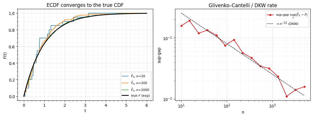
Left: the staircase tightens onto the smooth true CDF as grows. Right: the worst-case gap falls along the DKW line. So the ECDF is a consistent estimate of — the foundation under “rank-based” Gaussianization.
3. Rank → uniform → normal
Plugging the ECDF into the PIT gives the rank transform: a sample’s
uniform value is essentially its rank over , and of that is its
Gaussianized value. rbig.MarginalUniformize does the rank→uniform step and
rbig.MarginalGaussianize the whole rank→uniform→normal map; gauss_flows
splits it into a HistogramCDF (→ uniform) composed with InverseGaussCDF
(→ normal). We run the pipeline and check each stage.
u_rbig = rbig.MarginalUniformize().fit(x).transform(x)          # rank -> uniform
z_rbig = rbig.MarginalGaussianize().fit(x).transform(x)         # -> normal

hist = gf.HistogramCDF(n_bins=64, shape=(1,), method="linear").fit(jnp.asarray(x))
u_gf = np.asarray(jax.vmap(hist.transform)(jnp.asarray(x)))     # histogram -> uniform
z_gf = stats.norm.ppf(np.clip(u_gf, 1e-6, 1 - 1e-6))           # -> normal

fig, axes = plt.subplots(1, 3, figsize=(12, 3.6))
axes[0].hist(x[:, 0], bins=60, density=True, color="tab:blue", alpha=0.6)
axes[0].set(title="1. data $x$ (exponential)", xlabel="x", ylabel="density")
axes[1].hist(u_rbig[:, 0], bins=40, density=True, color="tab:orange", alpha=0.6)
axes[1].axhline(1.0, **GAUSS_KW, label="Uniform[0,1]")
axes[1].set(title=r"2. $u = \hat F(x)$ — uniform", xlabel="u"); axes[1].legend(fontsize=8)
zz = np.linspace(-4, 4, 200)
axes[2].hist(z_rbig[:, 0], bins=50, density=True, color="tab:green", alpha=0.6)
axes[2].plot(zz, stats.norm.pdf(zz), **GAUSS_KW, label=r"$\mathcal{N}(0,1)$")
axes[2].set(title=r"3. $z = \Phi^{-1}(u)$ — normal", xlabel="z"); axes[2].legend(fontsize=8)
for a in axes:
    style_ax(a)
fig.tight_layout()

print(f"rbig vs gauss_flows uniform stage agree: "
      f"max|Δ| = {np.max(np.abs(np.sort(u_rbig[:,0]) - np.sort(u_gf[:,0]))):.3f}")
rbig vs gauss_flows uniform stage agree: max|Δ| = 0.035
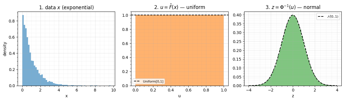
The exponential is pulled to a flat uniform and then to a clean bell — the PIT working through two different -estimators that agree closely. Note the price the ECDF pays at the edges, which the next section makes explicit.
4. The boundary problem (and support extension)
The ECDF assigns the largest sample and the smallest
, and it knows nothing beyond the observed range. Feed those
near- values to and the tail samples cannot be recovered on
the way back — the round-trip blows up (the failure of
Part 0 notebook 05). rbig’s
remedy is support extension (pdf_extension): pad the estimated density a
fraction of the data range past the extremes, giving the inverse room to place
tail samples instead of pinning them at the boundary.
for pe in [0.0, 0.1]:
    mu = rbig.MarginalUniformize(pdf_extension=pe).fit(x)
    err = np.abs(x - mu.inverse_transform(mu.transform(x))).max()
    print(f"pdf_extension = {pe:>4}:  round-trip max error = {err:.3e}")

mu0 = rbig.MarginalUniformize(pdf_extension=0.0).fit(x)
mu1 = rbig.MarginalUniformize(pdf_extension=0.1).fit(x)
err0 = np.abs(x - mu0.inverse_transform(mu0.transform(x))).ravel()
err1 = np.abs(x - mu1.inverse_transform(mu1.transform(x))).ravel()

fig, ax = plt.subplots(figsize=(7.5, 4))
order = np.argsort(x.ravel())
ax.semilogy(x.ravel()[order], np.maximum(err0[order], 1e-17), ".", ms=3,
            alpha=0.5, label="no support extension")
ax.semilogy(x.ravel()[order], np.maximum(err1[order], 1e-17), ".", ms=3,
            alpha=0.5, color="tab:green", label="pdf_extension = 0.1")
ax.set(title="Support extension rescues the tail-sample round-trip",
       xlabel="x (sample value)", ylabel="round-trip error")
ax.legend(); style_ax(ax)
fig.tight_layout()
pdf_extension = 0.0: round-trip max error = 7.616e-01
pdf_extension = 0.1: round-trip max error = 1.170e-02
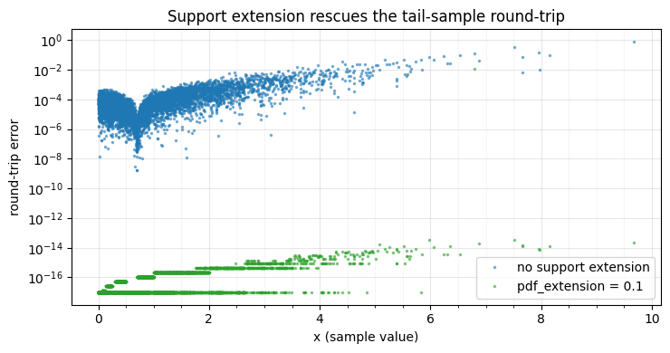
Support extension drops the worst-case round-trip error by ~60× (the spike is all at the largest samples). But it is a heuristic — a guess about mass past the data — and a rank/ECDF map is still piecewise constant between samples with no real tail model. That is the core limitation of empirical estimators, and the reason Part 1 now turns to smooth parametric CDFs.
5. The Jacobian: the gradient that becomes the log-det
A marginal earns its place in a flow only if we can compute its log-determinant — the per-coordinate gradient that change of variables (Part 0 00) turns into . For the chain rule gives
where is the estimated density and φ the standard-normal pdf — so a marginal’s log-det is its own density, in log space, re-referenced to the Gaussian. This exposes a second flaw in the pure ECDF: is a staircase, so its “density” is a sum of point masses — between samples and . The rank/ECDF transform Gaussianizes but has no usable Jacobian, so it is not a density model. The histogram CDF gives the first finite (if piecewise-constant) log-det.
xg = np.linspace(-4, 4, 800)[:, None]
u_h, log_f = jax.vmap(hist.transform_and_log_det)(jnp.asarray(xg))
u_h, log_f = np.asarray(u_h).ravel(), np.asarray(log_f).ravel()  # u=F(x), log_f=log f(x)
z_h = stats.norm.ppf(np.clip(u_h, 1e-6, 1 - 1e-6))
dzdx = np.exp(log_f) / stats.norm.pdf(z_h)                       # f(x) / phi(z)

fig, axes = plt.subplots(1, 2, figsize=(11, 4.2))
axes[0].plot(xg.ravel(), np.exp(log_f), color="tab:red", lw=1.5)
axes[0].set(title=r"histogram density $f(x)$ (piecewise constant)",
            xlabel="x", ylabel="$f(x)$")
style_ax(axes[0])
axes[1].plot(xg.ravel(), dzdx, color="tab:purple", lw=1.5)
axes[1].set(title=r"Jacobian $\mathrm{d}z/\mathrm{d}x = f(x)/\varphi(z)$",
            xlabel="x", ylabel=r"$\mathrm{d}z/\mathrm{d}x$")
style_ax(axes[1])
fig.tight_layout()
print("histogram Jacobian: finite but piecewise-constant; "
      "the bare ECDF would be 0 between samples -> log-det = -inf")
histogram Jacobian: finite but piecewise-constant; the bare ECDF would be 0 between samples -> log-det = -inf
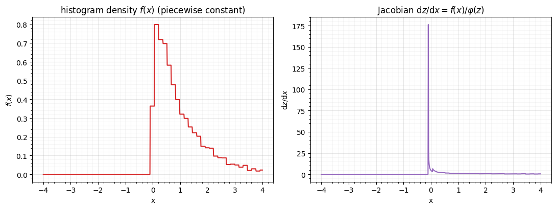
The density (left) is the staircase’s derivative — flat within each bin — and the Jacobian (right) inherits that bin structure, blowing up in the tails where . It is finite (unlike the ECDF’s), but jagged. A flow wants a smooth so the log-det is smooth and differentiable — exactly what the KDE and mixture/spline CDFs of the next notebooks provide.
Recap
| step | object | tool |
|---|---|---|
| rank → uniform | empirical CDF | rbig.MarginalUniformize, gf.HistogramCDF |
| uniform → normal | scipy/jax norm.ppf, gf.InverseGaussCDF | |
| full marginal map | rbig.MarginalGaussianize | |
| consistency | Glivenko–Cantelli / DKW | from scratch |
| tail fix | boundary correction, support extension | bound_correct, pdf_extension |
Next up. Empirical CDFs are consistent but jagged and tail-blind. 01 — KDE & Gaussian-mixture CDFs replaces the staircase with a smooth density estimate, giving an analytic, differentiable, tail-aware marginal transform.
- Dvoretzky, A., Kiefer, J., & Wolfowitz, J. (1956). Asymptotic Minimax Character of the Sample Distribution Function and of the Classical Multinomial Estimator. The Annals of Mathematical Statistics, 27(3), 642–669. 10.1214/aoms/1177728174