Fixed orthogonal & PCA warm starts
Freezing a PCA frame as a non-trainable rotation, and warm-starting a trainable Householder stack from a target Q
02 — Fixed orthogonal & PCA warm starts¶
Notebook 01 made the rotation trainable. But often the best rotation is one you do not train. The eigenvectors of the data covariance — the PCA frame — decorrelate the data in a single shot (notebook 00), so a sensible flow can freeze that frame and spend its parameters on the marginals instead. And when you do want a trainable rotation, you rarely want to start from scratch: initialising it at the PCA frame is a warm start that begins where the data already points.
This notebook covers both, with gauss_flows:
gf.FixedRotation.from_data— the decorrelating PCA rotation, held non-trainable so the optimiser cannot nudge it off the orthogonal manifold.- Why freezing matters — an unconstrained matrix trained by Adam drifts off , silently corrupting the flow’s log-det accounting.
- Warm-starting a trainable
gf.HouseholderRotationat a target via a closed-form Householder decomposition — reproducing the PCA frame exactly at initialisation, then fine-tuning from there.
What you will see
from_databuilds a pure rotation (orthogonal, log-det 0) whose rows are the principal axes, and it decorrelates the data.- A free matrix trained on a decorrelation proxy leaves — the failure
FixedRotation’sNonTrainablewrapper exists to prevent. - A Householder stack initialised from the decomposition matches the PCA frame to machine precision and then trains away from it freely.
import warnings

warnings.filterwarnings("ignore")

import equinox as eqx
import jax
import jax.numpy as jnp
import jax.random as jr
import matplotlib.pyplot as plt
import numpy as np
import optax

import gauss_flows as gf
from _style import SCATTER_KW, style_ax

jax.config.update("jax_enable_x64", True)
rng = np.random.default_rng(0)
1. The PCA frame as a fixed rotation¶
gf.FixedRotation.from_data(X) computes the eigenvectors of
and stores the orthogonal matrix whose rows are the principal axes, in
descending-eigenvalue order. The map is the decorrelating PCA
projection — a pure rotation, so and its log-det is exactly
0 (no whitening / rescale; that is left to the marginal step, cf.
notebook 00 §2). We fit it to a correlated cloud and
check it both rotates and decorrelates.
d = 3
n = 4000
M = jr.normal(jr.key(0), (d, d))
X = jr.normal(jr.key(1), (n, d)) @ M.T          # correlated, anisotropic

rot = gf.FixedRotation.from_data(X)
Q = np.asarray(rot.matrix)
Y = jax.vmap(rot.transform)(X)

x0 = jr.normal(jr.key(2), (d,))
z0, ld = rot.transform_and_log_det(x0)
xi, _ = rot.inverse_and_log_det(z0)
print(f"orthogonal? ||Q^T Q - I|| = {np.abs(Q.T @ Q - np.eye(d)).max():.1e}")
print(f"log_det = {float(ld):+.1e}   round-trip = {float(jnp.abs(x0 - xi).max()):.1e}")

cov_in = np.cov(np.asarray(X).T)
cov_out = np.cov(np.asarray(Y).T)
print(f"max |off-diagonal| covariance:  before = {np.abs(cov_in - np.diag(np.diag(cov_in))).max():.3f}"
      f"   after = {np.abs(cov_out - np.diag(np.diag(cov_out))).max():.2e}")

fig, axes = plt.subplots(1, 3, figsize=(14, 4.1))
axes[0].scatter(X[:, 0], X[:, 1], color="tab:blue", **SCATTER_KW)
axes[0].set(title="input (correlated)", xlabel="$x_0$", ylabel="$x_1$")
axes[1].scatter(Y[:, 0], Y[:, 1], color="tab:orange", **SCATTER_KW)
axes[1].set(title="after PCA frame $y=Qx$ (decorrelated)", xlabel="$y_0$", ylabel="$y_1$")
for ax in axes[:2]:
    ax.axhline(0, color="k", lw=0.6); ax.axvline(0, color="k", lw=0.6)
    ax.set_aspect("equal"); style_ax(ax)
im = axes[2].imshow(np.abs(cov_out), cmap="viridis")
axes[2].set(title="|Cov| after (diagonal)", xticks=range(d), yticks=range(d))
fig.colorbar(im, ax=axes[2], fraction=0.046)
fig.tight_layout()
orthogonal? ||Q^T Q - I|| = 8.9e-16
log_det = +0.0e+00 round-trip = 1.1e-15
max |off-diagonal| covariance: before = 0.753 after = 1.16e-15
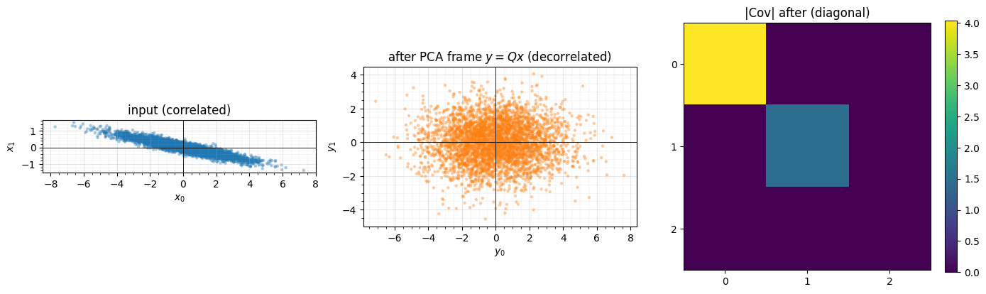
The frame rotates the cloud onto its principal axes and the output covariance is diagonal (off-diagonals drop from O(1) to ). Note it does not rescale — the axis variances are the eigenvalues, still unequal — which is exactly the point: the rotation decorrelates, the marginal step that follows it standardises. log-det stays 0.
2. Why freeze it¶
A PCA frame is fit once and should stay put. FixedRotation stores its matrix
wrapped in paramax.NonTrainable, so flowjax’s fit_to_data skips it
during gradient descent. That is not a cosmetic choice. If you instead expose the
rotation as a raw, unconstrained matrix and let Adam touch it, it drifts off the
orthogonal manifold — and then , so a flow that assumes
rotations contribute log-det 0 will silently mis-account the likelihood. We
demonstrate the drift on a decorrelation proxy.
Xc = X - X.mean(0)

def offdiag_loss_matrix(W):
    """Sum of squared off-diagonal covariance of W x — a decorrelation proxy."""
    C = (Xc @ W.T).T @ (Xc @ W.T) / n
    return jnp.sum((C - jnp.diag(jnp.diag(C))) ** 2)

W = jnp.asarray(Q)                                   # start at the (orthogonal) PCA frame
opt = optax.adam(2e-2)
state = opt.init(W)

@jax.jit
def step(W, state):
    loss, g = jax.value_and_grad(offdiag_loss_matrix)(W)
    upd, state = opt.update(g, state)
    return optax.apply_updates(W, upd), state, loss

ortho_err, logdets = [], []
for _ in range(400):
    W, state, _ = step(W, state)
    ortho_err.append(float(jnp.abs(W.T @ W - jnp.eye(d)).max()))
    logdets.append(float(jnp.linalg.slogdet(W)[1]))

print(f"unconstrained matrix after 400 steps:")
print(f"  ||W^T W - I|| = {ortho_err[-1]:.3f}   (left the orthogonal manifold)")
print(f"  log|det W|    = {logdets[-1]:+.3f}   (a flow would wrongly book this as 0)")

fig, ax = plt.subplots(figsize=(7.4, 4.2))
ax.plot(ortho_err, color="tab:red", lw=2, label=r"$\|W^\top W - I\|_\infty$ (orthogonality error)")
ax.plot(np.abs(logdets), color="tab:purple", lw=2, label=r"$|\log|\det W||$ (mis-booked log-det)")
ax.axhline(0, color="k", lw=0.8, ls="--")
ax.set(title="An unconstrained matrix drifts off $O(d)$ under training",
       xlabel="step", ylabel="error")
ax.legend(fontsize=8); style_ax(ax)
fig.tight_layout()
unconstrained matrix after 400 steps:
||W^T W - I|| = 0.221 (left the orthogonal manifold)
log|det W| = -0.158 (a flow would wrongly book this as 0)
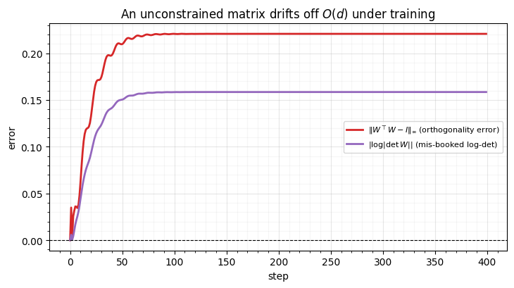
Starting exactly at the orthogonal PCA frame, the free matrix walks away from
within a few hundred steps — it “solves” the decorrelation proxy by
quietly rescaling, and now its true log-det is . FixedRotation avoids
this by freezing the frame; HouseholderRotation/OrthogonalRotation (notebook
- avoid it by parameterising orthogonality so every step stays on the manifold. The lesson: never train a rotation as a raw matrix. Either freeze it, or parameterise it.
This is the “fix the frame, learn the marginals” pattern: drop a
FixedRotation.from_data between marginal blocks and the rotation does its
decorrelating job for free while the trainable marginals do the standardising.
3. Warm-starting a trainable stack from a target ¶
What if we want the rotation trainable and want it to start at the PCA frame?
We need to set a HouseholderRotation’s reflection vectors so that its product
equals a given . That is a closed-form linear-algebra problem — the
Householder decomposition behind QR: zero out column by column with
reflections, then absorb the residual diagonal as axis reflections. The
reflectors satisfy .
def decompose_to_reflectors(Q):
    """Reflection vectors P such that gauss_flows' product H(P[-1])...H(P[0]) = Q.

    Column-by-column Householder zeroing reduces Q to a sign diagonal; each
    remaining -1 is one more axis reflection. Returns P ordered for gf's
    convention (gf applies reflections in array order, composing right-to-left).
    """
    Q = np.asarray(Q, float)
    d = Q.shape[0]
    R = Q.copy()
    us = []
    for k in range(d - 1):
        x = R[k:, k].copy()
        e = np.zeros_like(x); e[0] = 1.0
        alpha = -np.sign(x[0] or 1.0) * np.linalg.norm(x)   # stable sign choice
        v = x - alpha * e
        v = v / np.linalg.norm(v)
        u = np.zeros(d); u[k:] = v
        us.append(u)
        R[k:, k:] -= 2.0 * np.outer(v, v @ R[k:, k:])       # R <- H(v) R
    for j in np.where(np.sign(np.diag(R)) < 0)[0]:          # absorb the sign diagonal
        ej = np.zeros(d); ej[j] = 1.0
        us.append(ej)
    # H(us[-1])...H(us[0]) Q = I  =>  Q = H(us[0])...H(us[-1]); gf wants reversed order
    return np.array(us[::-1])

P = decompose_to_reflectors(Q)
warm = eqx.tree_at(lambda m: m.params,
                   gf.HouseholderRotation(n_reflections=P.shape[0], shape=(d,)),
                   jnp.asarray(P))
Q_warm = jax.vmap(warm.transform)(jnp.eye(d)).T
print(f"decomposed PCA frame into {P.shape[0]} reflections")
print(f"warm-started HouseholderRotation reproduces Q? ||Q - Q_warm|| = "
      f"{float(jnp.abs(jnp.asarray(Q) - Q_warm).max()):.1e}")
print(f"matches FixedRotation output on data? max|Δ| = "
      f"{float(jnp.abs(jax.vmap(warm.transform)(X) - Y).max()):.1e}")
decomposed PCA frame into 4 reflections
warm-started HouseholderRotation reproduces Q? ||Q - Q_warm|| = 4.4e-16
matches FixedRotation output on data? max|Δ| = 4.4e-15
The trainable stack now starts at the PCA frame to machine precision — it is
numerically identical to the FixedRotation, but its reflection vectors are
free to move. We contrast a cold start (random reflectors) against this
warm start while training the same decorrelation objective (now safely,
because the stack stays orthogonal at every step).
def offdiag_loss_layer(layer):
    Yl = jax.vmap(layer.transform)(Xc)
    C = Yl.T @ Yl / n
    return jnp.sum((C - jnp.diag(jnp.diag(C))) ** 2)

def train_layer(layer, steps=400, lr=2e-2):
    params, static = eqx.partition(layer, eqx.is_inexact_array)
    opt = optax.adam(lr); state = opt.init(params)

    @eqx.filter_jit
    def step(params, state):
        loss, g = eqx.filter_value_and_grad(
            lambda p: offdiag_loss_layer(eqx.combine(p, static)))(params)
        upd, state = opt.update(g, state)
        return eqx.apply_updates(params, upd), state, loss

    hist = []
    for _ in range(steps):
        params, state, loss = step(params, state)
        hist.append(float(loss))
    return hist

cold_hist = train_layer(gf.HouseholderRotation(n_reflections=d, shape=(d,)))
warm_hist = train_layer(warm)
print(f"cold start: off-diag loss {cold_hist[0]:.2e} -> {cold_hist[-1]:.2e}")
print(f"warm start: off-diag loss {warm_hist[0]:.2e} -> {warm_hist[-1]:.2e}  (begins at the answer)")

fig, ax = plt.subplots(figsize=(7.6, 4.3))
ax.semilogy(np.maximum(cold_hist, 1e-32), color="tab:blue", lw=2, label="cold start (random reflectors)")
ax.semilogy(np.maximum(warm_hist, 1e-32), color="tab:green", lw=2, label="warm start (PCA decomposition)")
ax.set(title="Warm-starting the rotation at the PCA frame",
       xlabel="step", ylabel="off-diagonal covariance loss")
ax.legend(fontsize=9); style_ax(ax)
fig.tight_layout()
cold start: off-diag loss 6.26e+00 -> 3.83e-19
warm start: off-diag loss 3.17e-30 -> 3.58e-19 (begins at the answer)
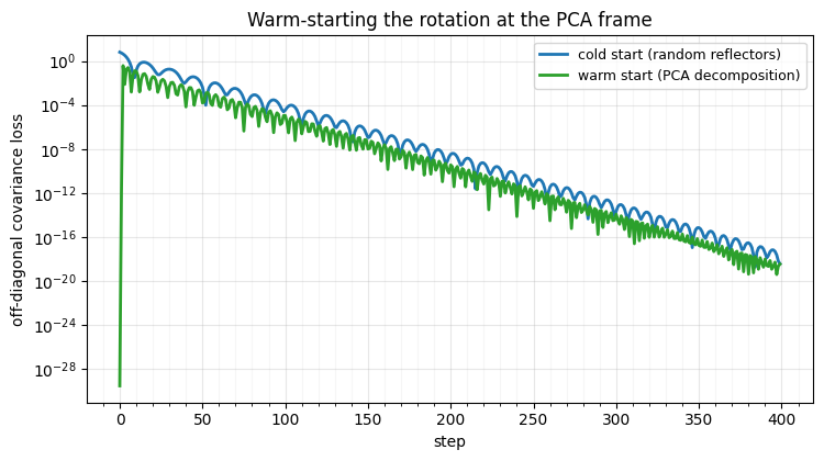
The warm-started stack begins already decorrelated (loss ) — it inherited the PCA solution — while the cold start has to descend from . Both reach machine zero, confirming the trainable stack can learn the frame; the warm start just gets it for free and then fine-tunes from a sensible place. This is the bridge between notebook 01’s trainable rotation and this notebook’s fixed one: decompose → initialise → fine-tune, the same recipe RBIG uses to warm-start parametric flows (Part 3).
Recap¶
| tool | rotation is | log-det | use when |
|---|---|---|---|
gf.FixedRotation.from_data | frozen PCA frame (NonTrainable) | 0 | fix the frame, learn only marginals |
| raw trainable matrix | drifts off | wrong | ✗ never — log-det silently corrupts |
gf.HouseholderRotation (warm-started) | trainable, init at | 0 | start at PCA, fine-tune by NLL |
The Householder decomposition turns any target — a PCA frame, a previous layer’s rotation — into an exact initialisation for a trainable stack.
Next up. Rotations are the dense orthogonal mixers. Image and high-dimensional flows need cheap structured linear layers with tractable log-dets: 03 — Structured linear layers covers the invertible convolution (LU-parameterised, ) and ActNorm, the data-dependent affine that makes deep stacks trainable.