Householder & trainable orthogonals

01 — Householder & trainable orthogonals¶

Notebook 00 fit a rotation once (PCA, ICA, random) and froze it. Inside a parametric Gaussianization flow we instead want to learn the rotation end-to-end, jointly with the marginal transforms, by gradient descent. That raises a problem: a rotation must satisfy $Q^\top Q = I$ , and an unconstrained matrix updated by SGD will not stay orthogonal. We need a parameterisation — a smooth map from free parameters $\theta\in\mathbb{R}^m$ to an orthogonal $Q(\theta)$ — that is orthogonal for every θ.

Two classic constructions do this, and gauss_flows ships both:

Products of Householder reflections — gf.HouseholderRotation, which spans the full orthogonal group $O(d)$ .
The Cayley map (and its cousin the matrix exponential) — gf.OrthogonalRotation, which spans the rotation subgroup $SO(d)$ .

Both keep $|\det Q| = 1$ exactly, so — echoing the “rotations are free” thread from Part 0 — the log-determinant they contribute stays exactly 0 at every gradient step.

What you will see

The Householder reflection from scratch: $H = I - 2vv^\top/\|v\|^2$ — a reflection across the hyperplane $\perp v$ , orthogonal with $\det = -1$ .
Why a product of reflections spans $O(d)$ , with $\det = (-1)^K$ .
Training the reflection vectors by gradient descent — orthogonality and log-det $=0$ hold at every step (no constraint, no projection).
The Cayley map and matrix exponential as the $SO(d)$ alternatives, and the precise reachability difference ( $O(d)$ vs $SO(d)$ ).

import warnings

warnings.filterwarnings("ignore")

import equinox as eqx
import jax
import jax.numpy as jnp
import jax.random as jr
import jax.scipy.linalg as jsl
import matplotlib.pyplot as plt
import numpy as np
import optax

import gauss_flows as gf
from _style import GAUSS_KW, style_ax

jax.config.update("jax_enable_x64", True)

1. The Householder reflection¶

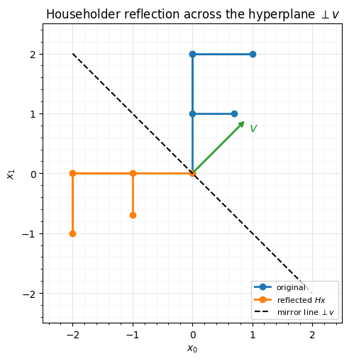
A Householder reflection is the simplest non-trivial orthogonal map. Given a unit vector $v$ , it reflects every point across the hyperplane through the origin orthogonal to $v$ :

H(v) = I - 2\,\frac{vv^\top}{\|v\|^2}.

((1))

It is orthogonal ( $H^\top H = I$ ), involutive ( $H^2 = I$ , a reflection undoes itself), and has $\det H = -1$ — it flips orientation. Here it is from scratch, reflecting a 2D shape across the line $\perp v$ .

def householder(v):
    """Householder reflector H = I - 2 v v^T / ||v||^2 for a vector v."""
    v = v / jnp.linalg.norm(v)
    return jnp.eye(v.shape[0]) - 2.0 * jnp.outer(v, v)

v2 = jnp.array([1.0, 1.0])              # reflect across the line perpendicular to (1,1)
H2 = householder(v2)
print(f"orthogonal? ||H^T H - I|| = {float(jnp.abs(H2.T @ H2 - jnp.eye(2)).max()):.1e}")
print(f"involutive? ||H@H - I||   = {float(jnp.abs(H2 @ H2 - jnp.eye(2)).max()):.1e}")
print(f"det H = {float(jnp.linalg.det(H2)):+.3f}  (reflection flips orientation)")

# An "F"-shaped point cloud so the reflection is visually obvious.
shape = np.array([[0, 0], [0, 2], [1, 2], [0, 2], [0, 1], [0.7, 1]], float).T
refl = np.asarray(H2 @ shape)

fig, ax = plt.subplots(figsize=(5.2, 5.2))
ax.plot(shape[0], shape[1], "o-", color="tab:blue", lw=2, label="original")
ax.plot(refl[0], refl[1], "o-", color="tab:orange", lw=2, label="reflected $Hx$")
tline = np.linspace(-2, 2, 2)
ax.plot(tline, -tline, **GAUSS_KW, label=r"mirror line $\perp v$")
ax.annotate("", xy=tuple(0.9 * np.asarray(v2)), xytext=(0, 0),
            arrowprops=dict(arrowstyle="->", color="tab:green", lw=2))
ax.text(0.95, 0.7, "$v$", color="tab:green", fontsize=13)
ax.set(title="Householder reflection across the hyperplane $\\perp v$",
       xlabel="$x_0$", ylabel="$x_1$", xlim=(-2.5, 2.5), ylim=(-2.5, 2.5))
ax.set_aspect("equal"); ax.legend(fontsize=8, loc="lower right"); style_ax(ax)
fig.tight_layout()

orthogonal? ||H^T H - I|| = 4.4e-16
involutive? ||H@H - I||   = 4.4e-16
det H = -1.000  (reflection flips orientation)

2. Products of reflections span $O(d)$ ¶

One reflection is not much, but products are everything: a classical theorem (the basis of the QR / Householder decomposition) says every orthogonal matrix in $O(d)$ is a product of at most $d$ Householder reflections. Stacking $K$ of them,

Q = H(v_K)\,H(v_{K-1})\cdots H(v_1), \qquad \det Q = (-1)^K,

((2))

gives an exactly-orthogonal $Q$ whose determinant is set by the parity of $K$ : odd $K$ → orientation-flipping ( $\det=-1$ ), even $K$ → a proper rotation ( $\det=+1$ ). gf.HouseholderRotation(n_reflections=K, shape=(d,)) is exactly this product, and — being orthogonal — its log-determinant is identically 0.

d = 3
x = jr.normal(jr.key(0), (d,))
for K in [1, 2, 3, 4]:
    b = gf.HouseholderRotation(n_reflections=K, shape=(d,))
    z, logdet = b.transform_and_log_det(x)
    xi, _ = b.inverse_and_log_det(z)
    # det of the effective matrix, from columns Q e_j
    Q = jax.vmap(b.transform)(jnp.eye(d))
    print(f"K={K}: log_det={float(logdet):+.1e}  det Q={float(jnp.linalg.det(Q)):+.2f}  "
          f"(-1)^K={(-1)**K:+d}  round-trip={float(jnp.abs(x - xi).max()):.1e}")

K=1: log_det=+0.0e+00  det Q=-1.00  (-1)^K=-1  round-trip=2.2e-16
K=2: log_det=+0.0e+00  det Q=+1.00  (-1)^K=+1  round-trip=3.1e-16
K=3: log_det=+0.0e+00  det Q=-1.00  (-1)^K=-1  round-trip=3.1e-16
K=4: log_det=+0.0e+00  det Q=+1.00  (-1)^K=+1  round-trip=3.1e-16

Every product is orthogonal to machine precision, log-det is exactly 0, and $\det Q$ tracks $(-1)^K$ . So to represent a general orthogonal map you take $K=d$ reflections; to guarantee a proper rotation you take an even $K$ . This is the workhorse trainable orthogonal in flow libraries (Householder flow, Tomczak & Welling (2016)).

3. Training the rotation, end-to-end¶

The point of a parameterisation is that its free parameters are unconstrained: any real values give a valid orthogonal $Q$ . So we can drop gf.HouseholderRotation straight into an optax loop and train it by plain gradient descent — no orthogonality constraint, no re-projection — with the log-det pinned at 0 the whole way. (The reflection of §1 was built by hand to see the construction; from here on we train the real gauss_flows layer.) We demonstrate by learning the rotation that reproduces a target $Q_\star$ .

One subtlety, straight from §2: a product of $K$ reflections has $\det = (-1)^K$ , so to fit a proper rotation ( $\det Q_\star = +1$ ) we must use an even number of reflections. We will return to what happens when the parity is wrong in §5 — it is not a bug, it is geometry.

def random_orthogonal(key, d, det=+1):
    """A random orthogonal matrix with a chosen determinant sign.

    QR of a Gaussian gives a Haar-random orthogonal Q; flipping a single column
    flips det(Q), which is the *correct* way to fix the sign for any d (scaling
    the whole matrix by -1 only flips the sign when d is odd).
    """
    Q, _ = jnp.linalg.qr(jr.normal(key, (d, d)))
    if float(jnp.linalg.det(Q)) * det < 0:
        Q = Q.at[:, 0].set(-Q[:, 0])
    return Q


def train_rotation(layer, Q_star, steps=1500, lr=5e-2):
    """Fit a gauss_flows orthogonal `layer` to a target matrix with optax.

    Returns (loss_history, logdet_history). The layer's effective matrix is
    Q = [T(e_1) ... T(e_d)]; we minimise ||Q - Q_star||^2 over its parameters.
    """
    d = Q_star.shape[0]
    I = jnp.eye(d)
    params, static = eqx.partition(layer, eqx.is_inexact_array)
    opt = optax.adam(lr)
    state = opt.init(params)

    def loss_fn(params):
        b = eqx.combine(params, static)
        Q = jax.vmap(b.transform)(I).T
        return jnp.sum((Q - Q_star) ** 2)

    @eqx.filter_jit
    def step(params, state):
        loss, g = eqx.filter_value_and_grad(loss_fn)(params)
        upd, state = opt.update(g, state)
        return eqx.apply_updates(params, upd), state, loss

    losses, logdets = [], []
    for _ in range(steps):
        params, state, loss = step(params, state)
        b = eqx.combine(params, static)
        losses.append(float(loss))
        logdets.append(float(b.transform_and_log_det(jnp.ones(d))[1]))
    return losses, logdets


Q_star = random_orthogonal(jr.key(1), d, det=+1)        # a proper rotation
hh_loss, hh_logdet = train_rotation(
    gf.HouseholderRotation(n_reflections=2, shape=(d,)), Q_star)   # even K -> det +1

print(f"target det = {float(jnp.linalg.det(Q_star)):+.2f}")
print(f"gf.HouseholderRotation (K=2) final fit ||Q - Q*||^2 = {hh_loss[-1]:.2e}")
print(f"max |log|det Q|| over training = {max(abs(x) for x in hh_logdet):.1e}  (stays 0)")

fig, (axL, axR) = plt.subplots(1, 2, figsize=(11, 4.2))
axL.semilogy(hh_loss, color="tab:purple", lw=2)
axL.set(title="Training gf.HouseholderRotation to match $Q_\\star$",
        xlabel="step", ylabel=r"$\|Q(\theta) - Q_\star\|^2$")
style_ax(axL)
axR.plot(hh_logdet, color="tab:green", lw=2, label=r"$\log|\det Q(\theta)|$")
axR.axhline(0, **GAUSS_KW)
axR.set(title="Orthogonality is free: log-det $\\equiv 0$ throughout",
        xlabel="step", ylabel=r"$\log|\det Q|$", ylim=(-1e-13, 1e-13))
axR.legend(fontsize=9); style_ax(axR)
fig.tight_layout()

target det = +1.00
gf.HouseholderRotation (K=2) final fit ||Q - Q*||^2 = 1.63e-31
max |log|det Q|| over training = 0.0e+00  (stays 0)

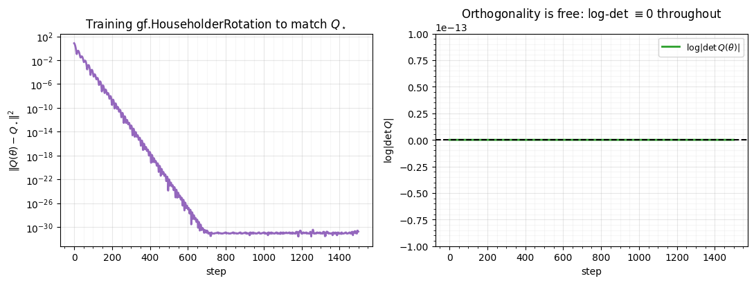
The fit drops to machine zero — two reflections reproduce the target rotation exactly — and the right panel is the headline: $\log|\det Q|$ never leaves 0 (to $\sim10^{-13}$ ). The optimiser walks freely through the unconstrained parameter space while $Q(\theta)$ stays glued to the orthogonal manifold. That is what makes it a free trainable rotation: it adds expressive mixing to a flow without ever charging the log-likelihood a log-det.

4. The Cayley map and the matrix exponential¶

Householder builds $Q$ from reflections. The other route builds it from a skew-symmetric matrix $A = -A^\top$ , which has exactly $d(d-1)/2$ free entries. Two maps send skew → orthogonal:

\textbf{Cayley:}\quad Q = (I - A)(I + A)^{-1}, \qquad \textbf{matrix exp:}\quad Q = \exp(A).

((3))

Both land in $SO(d)$ — $\det Q = +1$ always — and both are the identity at $A=0$ , the natural initialisation for a flow layer. We first confirm the two formulas really are orthogonal, then train gf.OrthogonalRotation (which uses the Cayley map — one linear solve, no matrix exponential) on the same target.

def skew(p):
    """Pack d(d-1)/2 free params into a skew-symmetric matrix A = -A^T."""
    A = jnp.zeros((d, d)).at[jnp.tril_indices(d, -1)].set(p)
    return A - A.T

p0 = jr.normal(jr.key(7), (d * (d - 1) // 2,))
A = skew(p0)
Q_cayley = jnp.linalg.solve(jnp.eye(d) + A, jnp.eye(d) - A)
Q_expm = jsl.expm(A)
print(f"Cayley : orthogonal? {float(jnp.abs(Q_cayley.T @ Q_cayley - jnp.eye(d)).max()):.1e}"
      f"   det = {float(jnp.linalg.det(Q_cayley)):+.3f}")
print(f"expm   : orthogonal? {float(jnp.abs(Q_expm.T @ Q_expm - jnp.eye(d)).max()):.1e}"
      f"   det = {float(jnp.linalg.det(Q_expm)):+.3f}")

o = gf.OrthogonalRotation(shape=(d,))
zo, ldo = o.transform_and_log_det(x)
print(f"gf.OrthogonalRotation: log_det={float(ldo):+.1e}, identity at init? {bool(jnp.allclose(zo, x))}")

oc_loss, oc_logdet = train_rotation(gf.OrthogonalRotation(shape=(d,)), Q_star)
print(f"gf.OrthogonalRotation final fit to the same Q_star = {oc_loss[-1]:.2e}"
      f"   (max |log-det| = {max(abs(x) for x in oc_logdet):.1e})")

Cayley : orthogonal? 3.3e-16   det = +1.000
expm   : orthogonal? 3.3e-16   det = +1.000
gf.OrthogonalRotation: log_det=+0.0e+00, identity at init? True

gf.OrthogonalRotation final fit to the same Q_star = 6.21e-22   (max |log-det| = 0.0e+00)

Both formulas are orthogonal to machine precision with $\det = +1$ , the Cayley OrthogonalRotation starts at the identity with log-det 0, and it fits the (proper-rotation) target to machine zero. So for a rotation, all three parameterisations are interchangeable — pick by cost: Cayley is one linear solve in $d(d-1)/2$ parameters, Householder is $K$ rank-one updates.

5. Which can reach what — the determinant-parity wall¶

There is one real difference, and it is about reachability. The Cayley map and matrix exponential only ever produce $\det = +1$ : they parameterise the rotation subgroup $SO(d)$ and cannot represent an orientation flip. A Householder product can — by using an odd number of reflections. We make the gap concrete by trying to fit a reflection ( $\det Q_\star = -1$ ) with each.

Q_ref = random_orthogonal(jr.key(1), d, det=-1)           # a reflection (det -1)
print(f"target is a reflection: det Q_ref = {float(jnp.linalg.det(Q_ref)):+.2f}\n")

hh_ref_loss, _ = train_rotation(gf.HouseholderRotation(n_reflections=3, shape=(d,)), Q_ref)  # odd K
oc_ref_loss, _ = train_rotation(gf.OrthogonalRotation(shape=(d,)), Q_ref)
print(f"gf.HouseholderRotation K=3 (odd, det -1): fit = {hh_ref_loss[-1]:.2e}   <- reaches the reflection")
print(f"gf.OrthogonalRotation  (SO(d), det +1)  : fit = {oc_ref_loss[-1]:.2e}   <- stuck at the parity wall")

target is a reflection: det Q_ref = -1.00

gf.HouseholderRotation K=3 (odd, det -1): fit = 4.78e-31   <- reaches the reflection
gf.OrthogonalRotation  (SO(d), det +1)  : fit = 4.00e+00   <- stuck at the parity wall

The Householder product nails the reflection; the Cayley map plateaus at $\|Q-Q_\star\|^2 = 4$ — the minimal distance between two orthogonal matrices of opposite determinant (it is $2d - 2\,\mathrm{tr}(Q^\top Q_\star)$ maximised over the wrong component). That flat plateau is not a local minimum or a tuning failure: no skew $A$ can give $\det = -1$ , so the target is simply unreachable. The same wall is why fitting a proper rotation needs an even number of reflections (§3): parity is geometry, not optimisation.

For a Gaussianization flow this rarely bites — a downstream sign flip in the marginal step absorbs orientation — but it is the precise mathematical reason HouseholderRotation (all of $O(d)$ ) and OrthogonalRotation (only $SO(d)$ ) are not interchangeable in general.

Recap¶

parameterisation	from	spans	det	cost	API
Householder product	$K$ reflection vectors	$O(d)$	$(-1)^K$	$K$ rank-1 updates	`gf.HouseholderRotation`
Cayley map	skew $A$	$SO(d)$	+1	one linear solve	`gf.OrthogonalRotation`
matrix exponential	skew $A$	$SO(d)$	+1	one $\exp$	(`jsl.expm`)

All three are orthogonal by construction, so they train under unconstrained gradient descent with the log-determinant pinned at 0 — a free, learnable mixing layer for a flow. The only catch is the determinant-parity wall: match the target’s orientation (even/odd reflections), or stay in $SO(d)$ on purpose.

Next up. Sometimes we do not want to learn the rotation — we want to fix it from the data (a PCA frame) and only learn the marginals, or warm-start a trainable stack from a target $Q$ . 02 — Fixed orthogonal & PCA warm starts covers gf.FixedRotation, the PCA frame, and how to initialise a Householder stack to match a given $Q$ .

References¶

Tomczak, J. M., & Welling, M. (2016). Improving Variational Auto-Encoders using Householder Flow. NeurIPS Workshop on Bayesian Deep Learning.