The rotation zoo, and why rotation matters

00 — The rotation zoo, and why rotation matters¶

Part 1 built the atomic operation of Gaussianization: turn one coordinate into a standard normal via $z_i = \Phi^{-1}(F_i(x_i))$ . But a stack of independent 1D maps can only ever fix the marginals. It cannot touch the dependence between coordinates — a product of per-axis maps is, by construction, separable. So if the data is correlated, marginal Gaussianization makes each axis look $\mathcal{N}(0,1)$ and then stalls, with the joint still far from $\mathcal{N}(0,I)$ .

The cure is the other half of Gaussianization: an orthogonal rotation between marginal passes, which mixes information across coordinates so the next marginal pass has something to do. Iterating (marginal → rotate → marginal → rotate …) is exactly RBIG Laparra et al. (2011). This notebook is the conceptual anchor for Part 2.

What you will see

The rotation zoo in rbig — PCA, ICA, random, Picard — and how they differ as orthogonal maps.
Why a pure rotation is free: $\log|\det Q| = 0$ (the Part 0 composition thread), while a whitening rotation pays a scaling log-det.
The headline demo: marginal-only Gaussianization stalls at high total correlation; inserting a rotation drives it to zero.
Rotation choice sets the convergence speed — PCA in one step, a random rotation in a few (previewing Part 3’s rotation studies).

import warnings

warnings.filterwarnings("ignore")

import jax
import matplotlib.pyplot as plt
import numpy as np

import rbig
from _style import SCATTER_KW, style_ax

jax.config.update("jax_enable_x64", True)
rng = np.random.default_rng(0)

1. The rotation zoo¶

A rotation here is an orthogonal linear map $z = Q x$ with $Q^\top Q = I$ . Orthogonality buys two things at once: it is exactly invertible ( $x = Q^\top z$ ), and — because $|\det Q| = 1$ — it is volume-preserving, so it contributes nothing to the change-of-variables log-determinant. rbig ships a whole zoo, differing only in how they pick $Q$ :

rotation	how $Q$ is chosen	when it shines
PCA	eigenvectors of $\mathrm{Cov}(X)$	scales differ across axes; decorrelates in one shot
ICA Hyvärinen & Oja (2000)	maximise non-Gaussianity of the axes	heavy-tailed / non-Gaussian structure
random	Haar-uniform $Q\sim O(d)$ via QR of a Gaussian	no fitting cost; the RBIG default guarantee
Picard Ablin et al. (2018)	quasi-Newton ICA on the orthogonal manifold	fast, robust ICA

Let’s fit each on a correlated, slightly non-Gaussian 2D cloud and look at the axes they choose.

# Correlated, mildly heavy-tailed 2D data: a shared latent + per-axis noise,
# stretched along a diagonal.
n = 4000
s = rng.standard_normal(n)
X = np.stack([2.0 * s + 0.6 * rng.standard_normal(n),
              1.2 * s + 0.6 * rng.standard_normal(n)], axis=1)

rotations = {
    "PCA": rbig.PCARotation(whiten=False),
    "ICA": rbig.ICARotation(random_state=0),
    "random": rbig.RandomRotation(random_state=0),
    "Picard": rbig.PicardRotation(random_state=0),
}

fig, axes = plt.subplots(1, 4, figsize=(15, 3.9), sharex=True, sharey=True)
for ax, (name, rot) in zip(axes, rotations.items()):
    rot.fit(X)
    Z = rot.transform(X)
    ax.scatter(Z[:, 0], Z[:, 1], color="tab:orange", **SCATTER_KW)
    ld = float(np.mean(rot.log_det_jacobian(X)))
    ax.set(title=f"{name}\nmean log|det J| = {ld:+.3f}", xlabel="$z_0$")
    ax.axhline(0, color="k", lw=0.6); ax.axvline(0, color="k", lw=0.6)
    style_ax(ax)
axes[0].set_ylabel("$z_1$")
fig.suptitle("The rotation zoo: same data, four orthogonal frames", y=1.02)
fig.tight_layout()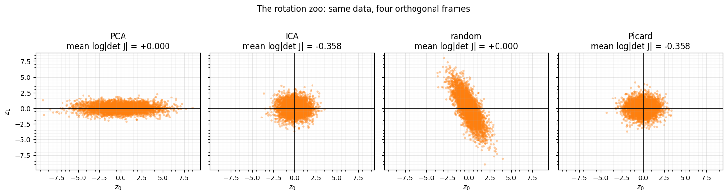

Each rotation re-expresses the same cloud in a different orthogonal frame. PCA aligns the axes with the directions of maximum variance (here the diagonal), so the cloud comes out axis-aligned. ICA and Picard instead hunt for the most non-Gaussian projections. Random just picks some Haar frame — no fitting at all. Crucially, all four are pure rotations: their mean log-determinant is 0.

2. A pure rotation is free; whitening is not¶

The log-det printed above was 0 because $|\det Q| = 1$ for an orthogonal $Q$ . That is the same fact Part 0 used to call rotations “free” inside a composed flow (composition log-det): a rotation re-frames the data without stretching volume, so it adds nothing to $\sum_k \log|\det J_k|$ . But beware — PCA-whitening is a rotation and a per-axis rescale ( $z = \Lambda^{-1/2} Q^\top x$ ), and that scaling is not free:

rot_only = rbig.PCARotation(whiten=False).fit(X)
whiten = rbig.PCARotation(whiten=True).fit(X)
print(f"PCA rotation only (whiten=False): mean log|det J| = "
      f"{np.mean(rot_only.log_det_jacobian(X)):+.4f}   <- free")
print(f"PCA whitening   (whiten=True):    mean log|det J| = "
      f"{np.mean(whiten.log_det_jacobian(X)):+.4f}   <- pays for the rescale")
print(f"  (the rescale contributes -sum(0.5*log(eigvals)) of Cov(X))")

PCA rotation only (whiten=False): mean log|det J| = +0.0000   <- free
PCA whitening   (whiten=True):    mean log|det J| = -0.3585   <- pays for the rescale
  (the rescale contributes -sum(0.5*log(eigvals)) of Cov(X))

So when Part 2 talks about “rotations are free”, it means the orthogonal part. A whitening step folds in a diagonal scaling whose log-det is $-\tfrac12\sum_i\log\lambda_i$ — cheap to compute, but not zero. Most RBIG variants keep the rotation pure and let the marginal step do the rescaling, which keeps the bookkeeping clean.

3. Why rotation matters: the stuck-vs-unstuck demo¶

Here is the whole reason Part 2 exists. Take strongly correlated data and run the marginal-Gaussianization step on its own, repeatedly. Then run it again with a rotation inserted between passes. We measure progress with the total correlation Watanabe (1960) $\mathrm{TC}(X) = \sum_i H(X_i) - H(X)$ — the multi-information that is 0 iff the coordinates are independent, and which rbig.total_correlation estimates directly.

def marginal_gaussianize(A):
    """One per-coordinate Gaussianization pass (the Part 1 atom)."""
    return rbig.MarginalGaussianize().fit(A).transform(A)

def total_corr(A):
    return float(rbig.total_correlation(A))

# Highly correlated, near-Gaussian data so that ONLY the dependence is the
# obstacle — marginals are already easy, the joint is not.
s = rng.standard_normal(n)
Xc = np.stack([s + 0.3 * rng.standard_normal(n),
               s + 0.3 * rng.standard_normal(n)], axis=1)

n_iter = 8
schemes = {
    "marginal only": None,
    "marginal + PCA rotation": lambda k: rbig.PCARotation(whiten=False),
    "marginal + random rotation": lambda k: rbig.RandomRotation(random_state=k),
}
histories = {}
for label, make_rot in schemes.items():
    A = Xc.copy()
    tc = [total_corr(A)]
    for k in range(n_iter):
        A = marginal_gaussianize(A)
        if make_rot is not None:
            A = make_rot(k).fit(A).transform(A)
        tc.append(total_corr(A))
    histories[label] = tc
    print(f"{label:28s} TC: " + " ".join(f"{v:5.3f}" for v in tc))

marginal only                TC: 0.922 0.925 0.925 0.925 0.925 0.925 0.925 0.925 0.925

marginal + PCA rotation      TC: 0.922 -0.003 0.000 -0.004 -0.000 0.000 0.000 0.000 0.000

marginal + random rotation   TC: 0.922 0.859 0.002 -0.002 0.001 -0.001 -0.000 -0.001 0.001

fig, (axL, axR) = plt.subplots(1, 2, figsize=(12, 4.4))

colors = {"marginal only": "tab:red",
          "marginal + PCA rotation": "tab:green",
          "marginal + random rotation": "tab:blue"}
for label, tc in histories.items():
    axL.plot(range(len(tc)), tc, "o-", color=colors[label], lw=2, ms=5, label=label)
axL.axhline(0, **{"color": "k", "lw": 1.5, "ls": "--"}, label="independent (TC = 0)")
axL.set(title="Marginal-only stalls; a rotation unsticks it",
        xlabel="iteration", ylabel="total correlation (nats)")
axL.legend(fontsize=8); style_ax(axL)

# Right: the geometry — marginal-only leaves a tilted Gaussian-on-the-diagonal.
A_marg = Xc.copy()
for _ in range(n_iter):
    A_marg = marginal_gaussianize(A_marg)
axR.scatter(A_marg[:, 0], A_marg[:, 1], color="tab:red", **SCATTER_KW,
            label="marginal-only (still correlated)")
A_rot = Xc.copy()
for k in range(n_iter):
    A_rot = marginal_gaussianize(A_rot)
    A_rot = rbig.PCARotation(whiten=False).fit(A_rot).transform(A_rot)
axR.scatter(A_rot[:, 0], A_rot[:, 1], color="tab:green", **SCATTER_KW,
            label="marginal + rotation (isotropic)")
axR.set(title="The joint after 8 passes", xlabel="$z_0$", ylabel="$z_1$",
        xlim=(-4, 4), ylim=(-4, 4))
axR.axhline(0, color="k", lw=0.6); axR.axvline(0, color="k", lw=0.6)
axR.legend(fontsize=8, loc="upper left"); style_ax(axR)
fig.tight_layout()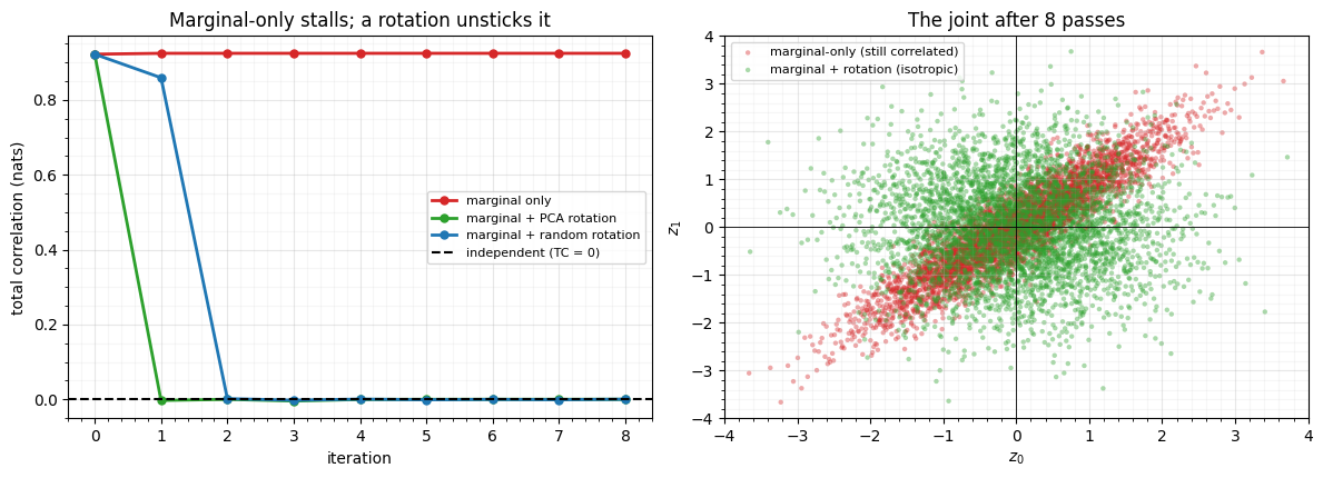

Marginal-only (red) is stuck. Each pass dutifully makes both axes $\mathcal{N}(0,1)$ , but a separable map can never remove the diagonal correlation, so the total correlation plateaus around 0.9 nats forever — the scatter stays a tilted ellipse pinned to the diagonal. A separable transform has a separable image; you cannot reach $\mathcal{N}(0,I)$ this way.

Insert a rotation and the obstacle dissolves. The rotation mixes the two coordinates, so the next marginal pass sees fresh non-Gaussian structure to remove. With PCA the data is near-Gaussian, so a single decorrelating rotation collapses TC to 0 in one step. A random rotation has no idea where the correlation lives, so it takes a couple of passes — but it does converge. That robustness is the theoretical heart of RBIG Laparra et al. (2011): for near-Gaussian targets almost any rotation works, because each marginal pass can only reduce the total correlation and a generic rotation keeps exposing reducible structure.

4. Rotation choice sets the convergence speed¶

The demo already hints at it: PCA reached independence in one step, random in two. That difference — same destination, different speed — is what makes rotation choice a real design knob. We make it explicit by counting passes to drive TC below a tolerance.

tol = 1e-2
print(f"passes to reach TC < {tol}:")
for label, tc in histories.items():
    if label == "marginal only":
        print(f"  {label:28s} never (plateau at {tc[-1]:.3f})")
        continue
    hit = next((i for i, v in enumerate(tc) if abs(v) < tol), None)
    print(f"  {label:28s} {hit} passes")

passes to reach TC < 0.01:
  marginal only                never (plateau at 0.925)
  marginal + PCA rotation      1 passes
  marginal + random rotation   2 passes

PCA wins here because the data is Gaussian and correlated — exactly the case its eigenvector frame is built for. On heavy-tailed or multimodal data, ICA and Picard can win instead by aligning to the non-Gaussian directions, while random is the safe, fit-free default whose only cost is a few extra passes. Part 3 turns this into a proper rotation-choice convergence study; here the point is simply that the between-coordinate step is not an afterthought — it is half the algorithm.

Recap¶

idea	takeaway
rotation = orthogonal map $z = Qx$	exactly invertible, volume-preserving ($\log
marginal-only Gaussianization	fixes marginals, cannot remove dependence — stalls
rotation between passes	mixes coordinates so the next marginal pass progresses → TC $\to 0$
rotation choice	sets convergence speed: PCA (variance), ICA/Picard (non-Gaussianity), random (free, robust)
whitening ≠ pure rotation	the rescale costs a $-\tfrac12\sum\log\lambda_i$ log-det

Next up. A random or PCA rotation is fixed once fit. To learn the rotation end-to-end inside a flow we need an orthogonal matrix that stays orthogonal under gradient descent. 01 — Householder & trainable orthogonals builds two such parameterisations from scratch — products of Householder reflections and the Cayley map — both exactly orthogonal, both with log-det 0.

References¶

Laparra, V., Camps-Valls, G., & Malo, J. (2011). Iterative Gaussianization: From ICA to Random Rotations. IEEE Transactions on Neural Networks, 22(4), 537–549. 10.1109/TNN.2011.2106511
Hyvärinen, A., & Oja, E. (2000). Independent Component Analysis: Algorithms and Applications. Neural Networks, 13(4–5), 411–430.
Ablin, P., Cardoso, J.-F., & Gramfort, A. (2018). Faster Independent Component Analysis by Preconditioning with Hessian Approximations. IEEE Transactions on Signal Processing, 66(15), 4040–4049.
Watanabe, S. (1960). Information Theoretical Analysis of Multivariate Correlation. IBM Journal of Research and Development, 4(1), 66–82. 10.1147/rd.41.0066