Structured linear layers: 1×1 conv & ActNorm

03 — Structured linear layers: 1×1 conv & ActNorm¶

Notebooks 00–02 covered orthogonal mixers: rotations, which are volume-preserving ( $\log|\det| = 0$ ). But the “between-coordinate” toolkit has two more members, both introduced by Glow Kingma & Dhariwal (2018), that are general linear maps — not orthogonal, so they carry a real log-det — yet keep that log-det cheap ( $O(d)$ instead of $O(d^3)$ ) by construction:

The invertible $1\times1$ convolution — a learnable dense channel mixer $y = Wx$ , stored in LU form so $\log|\det W| = \sum\log|s|$ .
ActNorm — a per-channel affine $y = (x-b)/s$ with a data-dependent initialisation that standardises activations and makes deep stacks trainable.

Together with coupling layers, these are the repeating unit of a Glow step (ActNorm → $1\times1$ conv → coupling). Here we build the two linear pieces with gauss_flows.

What you will see

The $1\times1$ conv as a per-pixel channel mixer, with $\log|\det W| = \sum\log|s|$ verified against the dense determinant.
Why LU matters: the map stays exactly invertible under training, where a raw matrix (notebook 02) would drift singular.
ActNorm’s data-dependent init from a batch — output mean $\approx 0$ , std $\approx 1$ per channel — and why that conditioning helps depth.

import warnings

warnings.filterwarnings("ignore")

import equinox as eqx
import jax
import jax.numpy as jnp
import jax.random as jr
import matplotlib.pyplot as plt
import numpy as np
import optax

import gauss_flows as gf
from _style import style_ax

jax.config.update("jax_enable_x64", True)
rng = np.random.default_rng(0)

1. The invertible $1\times1$ convolution¶

A $1\times1$ convolution applies the same linear map $W$ to the channel vector at every spatial location: $y_{ij} = W x_{ij}$ , $W\in\mathbb{R}^{C\times C}$ . It is the learnable generalisation of the fixed channel permutation that RealNVP used to shuffle coordinates between coupling layers — instead of a hard permutation, a soft, trainable mixing. gf.Invertible1x1Conv operates on one channel vector $(C,)$ ; we vmap it across the spatial grid.

C = 4
conv = gf.Invertible1x1Conv(jr.key(0), n_channels=C)

# Make the log-det non-trivial by setting the U-diagonal (log s); near-identity
# at init otherwise. Its parameters are L (unit-diag), U (positive-diag = exp(log_diag_u)).
conv = eqx.tree_at(lambda m: m.log_diag_u, conv, jnp.array([0.5, -0.3, 0.2, 0.1]))

W = jax.vmap(conv.transform)(jnp.eye(C)).T          # effective matrix W (columns W e_j)
xch = jr.normal(jr.key(1), (C,))
z, ld = conv.transform_and_log_det(xch)
xi, _ = conv.inverse_and_log_det(z)

print(f"log_det (analytic, = sum log|s|) = {float(ld):+.4f}")
print(f"sum(log_diag_u)                  = {float(jnp.sum(jnp.array([0.5,-0.3,0.2,0.1]))):+.4f}")
print(f"log|det W| (dense, O(d^3))       = {float(jnp.linalg.slogdet(W)[1]):+.4f}")
print(f"round-trip = {float(jnp.abs(xch - xi).max()):.1e}")

# Apply across an 8x8 feature map: same W at every pixel, log-det adds up.
img = jr.normal(jr.key(2), (C, 8, 8))
flat = img.reshape(C, -1).T                          # (pixels, C)
z_pix = jax.vmap(conv.transform)(flat)
ld_pix = jax.vmap(lambda p: conv.transform_and_log_det(p)[1])(flat)
print(f"\non an 8x8 map: total log-det = {float(ld_pix.sum()):.3f} "
      f"= {float(ld):.3f} x {flat.shape[0]} pixels")

# Show the LU structure and the resulting W.
P, Lmat, Umat = jax.scipy.linalg.lu(np.asarray(W))
fig, axes = plt.subplots(1, 3, figsize=(12, 3.6))
for ax, Mx, name in zip(axes, [Lmat, Umat, W], ["L (unit diag)", "U (s = diag)", "W = LU"]):
    im = ax.imshow(np.asarray(Mx), cmap="RdBu_r", vmin=-1.5, vmax=1.5)
    ax.set(title=name, xticks=range(C), yticks=range(C))
    fig.colorbar(im, ax=ax, fraction=0.046)
fig.suptitle("1×1 conv weight stored in LU form — log|det W| = sum log|diag U|", y=1.04)
fig.tight_layout()

log_det (analytic, = sum log|s|) = +0.5000
sum(log_diag_u)                  = +0.5000
log|det W| (dense, O(d^3))       = +0.5000
round-trip = 2.2e-16


on an 8x8 map: total log-det = 32.000 = 0.500 x 64 pixels

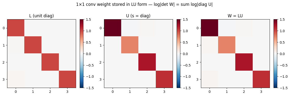
The analytic log-det matches the dense $\log|\det W|$ exactly, and round-trip is machine-precision. Across the $8\times8$ map the per-pixel log-det simply multiplies by the number of positions (64). Unlike a rotation, $W$ is a general linear map, so its log-det is non-zero — but reading it off the triangular factor’s diagonal costs $O(d)$ , not the $O(d^3)$ of a dense determinant.

2. Why LU: invertible by construction, cheap log-det¶

Two problems with learning a raw weight $W$ : (i) computing $\log|\det W|$ at every step is $O(d^3)$ , and (ii) nothing keeps $W$ invertible — gradient steps can drive it singular, and notebook 02 §2 showed an unconstrained matrix drifting off the manifold entirely. The LU parameterisation $W = LU$ fixes both: $L$ is unit-lower-triangular, $U$ is upper-triangular with $\mathrm{diag}(U) = \exp(\text{log\_diag\_u}) > 0$ , so $W$ is always invertible and $\log|\det W| = \sum_i \text{log\_diag\_u}_i$ is read straight off. We confirm it survives training intact, on an arbitrary objective.

batch = jr.normal(jr.key(3), (2000, C)) * jnp.array([3.0, 0.5, 2.0, 1.0])

def loss_fn(layer):
    Y = jax.vmap(layer.transform)(batch)
    return jnp.mean((jnp.sum(Y ** 2, axis=1) - C) ** 2)   # arbitrary, just to move params

conv0 = gf.Invertible1x1Conv(jr.key(0), n_channels=C)
params, static = eqx.partition(conv0, eqx.is_inexact_array)
opt = optax.adam(1e-2)
state = opt.init(params)

@eqx.filter_jit
def step(params, state):
    loss, g = eqx.filter_value_and_grad(lambda p: loss_fn(eqx.combine(p, static)))(params)
    upd, state = opt.update(g, state)
    return eqx.apply_updates(params, upd), state, loss

for _ in range(300):
    params, state, _ = step(params, state)
trained = eqx.combine(params, static)

W_t = jax.vmap(trained.transform)(jnp.eye(C)).T
ld_t = float(trained.transform_and_log_det(batch[0])[1])
x = batch[0]; xi_t, _ = trained.inverse_and_log_det(trained.transform(x))
print("after 300 training steps:")
print(f"  analytic log_det = {ld_t:+.4f}   dense log|det W| = {float(jnp.linalg.slogdet(W_t)[1]):+.4f}  (match)")
print(f"  round-trip       = {float(jnp.abs(x - xi_t).max()):.1e}  (still exactly invertible)")
print(f"  det W            = {float(jnp.linalg.det(W_t)):+.4f}  (never crossed 0)")

after 300 training steps:
  analytic log_det = -2.2268   dense log|det W| = -2.2268  (match)
  round-trip       = 2.2e-16  (still exactly invertible)
  det W            = +0.1079  (never crossed 0)

The analytic and dense log-dets stay equal, the round-trip stays at machine precision, and $\det W$ never approaches 0: the LU form keeps the layer a valid bijector for free, the structured counterpart to the orthogonal parameterisations of notebook 01. That is the whole reason flows store linear layers factored rather than dense.

3. ActNorm — data-dependent affine¶

ActNorm is the simplest structured layer: a per-channel affine $y = (x - b)\,/\,s$ with learnable location $b$ and positive scale $s = \mathrm{softplus}(\text{log\_scale}) + 10^{-5}$ . Its log-det is $-\sum_c \log s_c$ (times the number of spatial positions for an image). The trick that gives it its name is the data-dependent initialisation: set $b$ and $s$ from the first batch’s per-channel mean and std, so the layer’s output starts standardised — zero mean, unit variance per channel. That conditioning is what lets very deep stacks train without the activations exploding or collapsing.

gauss_flows exposes the parameters but not a from_data factory (unlike FixedRotation.from_data), so we write the three-line init ourselves.

def actnorm_from_data(batch):
    """Data-dependent ActNorm init: loc = per-channel mean, scale = per-channel std."""
    mu = batch.mean(axis=0)
    sd = batch.std(axis=0)
    inv_softplus = lambda y: jnp.log(jnp.expm1(y))            # softplus^{-1}
    log_scale = inv_softplus(jnp.clip(sd - 1e-5, 1e-6))
    layer = gf.ActNorm(shape=(batch.shape[1],))
    return eqx.tree_at(lambda m: (m.loc, m.log_scale), layer, (mu, log_scale))

# A batch with very different per-channel mean/scale.
raw = jr.normal(jr.key(4), (2000, C)) * jnp.array([3.0, 0.5, 2.0, 1.0]) + jnp.array([5.0, -2.0, 0.0, 1.0])

default_out = jax.vmap(gf.ActNorm(shape=(C,)).transform)(raw)     # log_scale = 0 -> scale ~ 0.69
datainit = actnorm_from_data(raw)
datainit_out = jax.vmap(datainit.transform)(raw)

print("per-channel statistics of the output:")
print(f"  default init : mean {np.round(np.asarray(default_out.mean(0)), 2)}  std {np.round(np.asarray(default_out.std(0)), 2)}")
print(f"  data init    : mean {np.round(np.asarray(datainit_out.mean(0)), 2)}  std {np.round(np.asarray(datainit_out.std(0)), 2)}")

fig, axes = plt.subplots(1, 2, figsize=(11, 4.0), sharey=True)
for c in range(C):
    axes[0].hist(np.asarray(raw[:, c]), bins=50, alpha=0.5, label=f"ch {c}")
    axes[1].hist(np.asarray(datainit_out[:, c]), bins=50, alpha=0.5, label=f"ch {c}")
axes[0].set(title="raw activations (heterogeneous scale/shift)", xlabel="value", ylabel="count")
axes[1].set(title="after data-init ActNorm (standardised)", xlabel="value")
for ax in axes:
    ax.legend(fontsize=8); style_ax(ax)
fig.tight_layout()

per-channel statistics of the output:
  default init : mean [ 7.05 -2.88  0.04  1.4 ]  std [4.3  0.71 2.89 1.46]
  data init    : mean [ 0.  0.  0. -0.]  std [1. 1. 1. 1.]

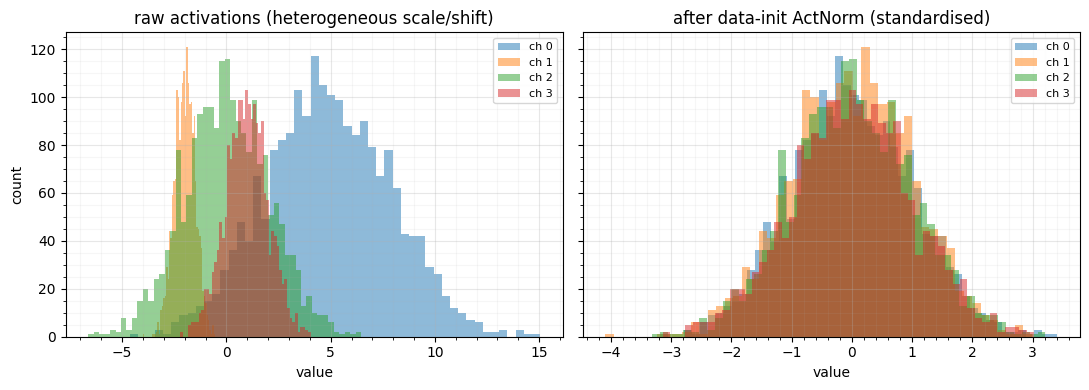
The default ActNorm (with log_scale = 0) just divides every channel by $\mathrm{softplus}(0)\approx0.69$ — it ignores the data’s wildly different per-channel scales and offsets. The data-initialised ActNorm pins every channel to mean $\approx 0$ , std $\approx 1$ , so the next layer sees well-conditioned inputs. Stacked through a deep flow, this is the difference between a network that trains and one whose log-likelihood diverges in the first few steps.

4. How they fit together¶

A Glow “step” is exactly these pieces in sequence: ActNorm preconditions the activations, the $1\times1$ conv mixes channels (replacing RealNVP’s fixed permutation), and a coupling layer (Part 5) does the expressive nonlinear work. All three have triangular or diagonal Jacobians, so their log-dets are $O(d)$ and simply add (Part 0 composition). The orthogonal mixers of notebooks 00–02 slot into the same position as the $1\times1$ conv — the choice is orthogonal (log-det 0, volume-preserving) versus general linear (log-det $\sum\log|s|$ , can rescale).

Recap¶

layer	map	log-det	kept valid by	API
rotation (nb 00–02)	$Qx$ , orthogonal	0	orthogonal parameterisation	`gf.HouseholderRotation`, …
$1\times1$ conv	$Wx$ , general linear	$\sum\log	s	$
ActNorm	$(x-b)/s$ , diagonal affine	$-\sum\log s$	positive scale, data init	`gf.ActNorm` / `ActNorm1D`

Rotations re-frame without rescaling; the $1\times1$ conv adds learnable rescaling with a cheap log-det; ActNorm adds the data-dependent conditioning that makes depth trainable. That completes the between-coordinate toolkit.

Next up — Part 3. With marginal transforms (Part 1) and orthogonal/linear mixers (Part 2) in hand, we can assemble the classic algorithm that alternates them to convergence: Rotation-Based Iterative Gaussianization (RBIG) — the non-parametric loop marginal → rotate → marginal → rotate … that drives a distribution to $\mathcal{N}(0,I)$ , with negentropy as its stopping signal.

References¶

Kingma, D. P., & Dhariwal, P. (2018). Glow: Generative Flow with Invertible 1x1 Convolutions. Advances in Neural Information Processing Systems (NeurIPS).