The Hutchinson trace estimator

01 — The Hutchinson trace estimator¶

In 00 — FFJORD the log-density of a continuous flow was a line integral of the trace of the Jacobian,

\log p_0(x_0) = \log p_1(x_1) + \int_0^1 \operatorname{tr}\!\big(\partial_x f_\theta(t, x_t)\big)\,\mathrm{d}t .

((1))

That trace is the continuous flow’s entire log-det machinery — and it is what makes CNFs scale or not. Computing $\operatorname{tr}(\partial_x f)$ exactly means extracting the $d$ diagonal entries of the $d\times d$ Jacobian, which costs $d$ Jacobian-vector products (one per coordinate) at every ODE step. In 2-D that is nothing; for a $32\times32\times3$ image ( $d=3072$ ) it is 3072 JVPs per step per sample — hopeless.

Hutchinson’s identity Hutchinson (1990) rescues it. For any random vector $z$ with $\mathbb{E}[z z^\top] = I$ ,

\operatorname{tr}(A) = \mathbb{E}_z\big[z^\top A z\big],

((2))

so a single probe gives an unbiased estimate of the trace from one Jacobian-vector product $Az = (\partial_x f)\,z$ — $O(1)$ per step instead of $O(d)$ . The price is variance: the estimate is noisy, shrinking as $1/\sqrt{n}$ in the number of probes $n$ . This is the trade FFJORD Grathwohl et al. (2019) makes to train free-form vector fields at scale.

What you will see

Hutchinson on a known matrix: unbiasedness and $1/\sqrt{n}$ convergence.
Rademacher vs Gaussian probes and the variance formulas — why Rademacher wins.
The estimator inside FFJORD: per-step divergence and the integrated-log-det error vs probe count, on a real gf.FFJORD.
Why the probes are fixed per instance (deterministic log-det → stable training).
The $O(d)$ vs $O(n)$ cost scaling — the reason continuous flows scale.

import warnings

warnings.filterwarnings("ignore")

import time

import equinox as eqx
import jax
import jax.numpy as jnp
import jax.random as jr
import matplotlib.pyplot as plt
import numpy as np
import optax
from flowjax.distributions import Normal, Transformed
from flowjax.train import fit_to_data

import gauss_flows as gf
from gauss_flows._src._divergence import exact_divergence, hutchinson_divergence
from _style import DATA_COLOR, GAUSS_KW, LATENT_COLOR, style_ax

jax.config.update("jax_enable_x64", True)

1. Hutchinson on a known matrix¶

Strip away the flow and look at the estimator on a fixed matrix $A$ where we know the answer. With $z$ a random sign vector (Rademacher, $z_i\in\{\pm1\}$ ), $z^\top A z = \sum_{i,j} A_{ij} z_i z_j$ . Taking expectations, the off-diagonal terms vanish ( $\mathbb{E}[z_i z_j]=0$ for $i\ne j$ ) and the diagonal terms survive ( $z_i^2 = 1$ ), leaving exactly $\sum_i A_{ii} = \operatorname{tr}(A)$ . The $n$ -probe estimator averages $n$ such draws.

d = 24
key = jr.key(0)
A_key, _ = jr.split(key)
# A symmetric matrix with a known trace.
M = jr.normal(A_key, (d, d))
A = 0.5 * (M + M.T)
tr_exact = float(jnp.trace(A))


def hutch_estimate(A, Z):
    """n-probe Hutchinson estimate from probes Z of shape (n, d): mean_k z_k^T A z_k."""
    return jnp.mean(jnp.sum((Z @ A) * Z, axis=1))


def rademacher(key, n, d):
    return jnp.sign(jr.normal(key, (n, d)))


# One probe at a time: unbiased but noisy.
single = jnp.array([hutch_estimate(A, rademacher(jr.key(s), 1, d)) for s in range(2000)])
print(f"exact trace                         = {tr_exact:+.4f}")
print(f"mean of 2000 single-probe estimates = {float(single.mean()):+.4f}  (unbiased)")
print(f"std  of single-probe estimates      = {float(single.std()):.4f}   (the noise to beat)")

exact trace                         = -2.7480
mean of 2000 single-probe estimates = -2.8666  (unbiased)

std  of single-probe estimates      = 21.7016   (the noise to beat)

The single-probe estimate is centered on the true trace but scatters widely. The $n$ -probe estimator averages that noise down. We sweep $n$ and measure the RMSE over many independent estimators, expecting the classic Monte-Carlo $1/\sqrt{n}$ .

probe_counts = np.array([1, 2, 4, 8, 16, 32, 64, 128, 256, 512])
n_trials = 400


def rmse_vs_n(sampler):
    out = []
    for i, n in enumerate(probe_counts):
        ests = jnp.array([
            hutch_estimate(A, sampler(jr.key(1000 * i + t), int(n), d))
            for t in range(n_trials)
        ])
        out.append(float(jnp.sqrt(jnp.mean((ests - tr_exact) ** 2))))
    return np.array(out)


rmse_rad = rmse_vs_n(rademacher)

fig, ax = plt.subplots(figsize=(6.2, 4.2))
ax.loglog(probe_counts, rmse_rad, "o-", color=DATA_COLOR, label="Rademacher RMSE")
ref = rmse_rad[0] / np.sqrt(probe_counts / probe_counts[0])
ax.loglog(probe_counts, ref, "k:", alpha=0.6, label=r"$\propto 1/\sqrt{n}$")
ax.set(xlabel="number of probes $n$", ylabel="RMSE of trace estimate",
       title="Hutchinson estimator converges as $1/\\sqrt{n}$")
ax.legend()
style_ax(ax)
fig.tight_layout()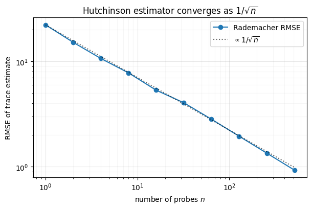

The RMSE rides the $1/\sqrt{n}$ reference exactly: quadrupling the probes halves the error. There is no bias to worry about — only this variance, which is why the probe distribution matters.

2. Rademacher vs Gaussian probes¶

Any $z$ with $\mathbb{E}[zz^\top]=I$ works, but they do not all have the same variance. For a symmetric $A$ ,

\operatorname{Var}_{\mathcal{N}}\!\big[z^\top A z\big] = 2\,\lVert A\rVert_F^2, \qquad \operatorname{Var}_{\text{Rad}}\!\big[z^\top A z\big] = 2\Big(\lVert A\rVert_F^2 - \textstyle\sum_i A_{ii}^2\Big).

((3))

The Rademacher variance is the Gaussian variance minus the diagonal’s contribution: because $z_i^2=1$ is deterministic for sign probes, the diagonal of $A$ (which is exactly what we are summing) carries no variance. That makes Rademacher the minimum-variance probe Hutchinson (1990), and the default in gauss_flows. We verify both formulas.

def gaussian(key, n, d):
    return jr.normal(key, (n, d))


fro2 = float(jnp.sum(A**2))
diag2 = float(jnp.sum(jnp.diag(A) ** 2))
var_formula = {"rademacher": 2 * (fro2 - diag2), "normal": 2 * fro2}

print(f"{'probe':>12s}  {'empirical var':>14s}  {'formula':>12s}")
for name, sampler in (("rademacher", rademacher), ("normal", gaussian)):
    s = jnp.array([hutch_estimate(A, sampler(jr.key(t), 1, d)) for t in range(4000)])
    print(f"{name:>12s}  {float(s.var()):>14.3f}  {var_formula[name]:>12.3f}")
print(f"\n(the diagonal adds 2*sum(A_ii^2) = {2 * diag2:.1f} to the Gaussian variance; "
      f"Rademacher avoids it entirely)")

rmse_norm = rmse_vs_n(gaussian)
fig, ax = plt.subplots(figsize=(6.2, 4.2))
ax.loglog(probe_counts, rmse_rad, "o-", color=DATA_COLOR, label="Rademacher")
ax.loglog(probe_counts, rmse_norm, "s--", color=LATENT_COLOR, label="Gaussian")
ax.set(xlabel="number of probes $n$", ylabel="RMSE of trace estimate",
       title="Rademacher beats Gaussian at every probe count")
ax.legend()
style_ax(ax)
fig.tight_layout()

       probe   empirical var       formula

  rademacher         486.031       483.506

      normal         532.999       540.290

(the diagonal adds 2*sum(A_ii^2) = 56.8 to the Gaussian variance; Rademacher avoids it entirely)

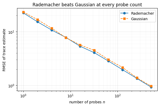
The empirical variances match the formulas, and Rademacher sits below Gaussian at every $n$ — same cost, less noise. (For a general non-symmetric $A$ , as the flow Jacobian will be, the constants change but Rademacher’s diagonal-is-free advantage remains.)

3. The estimator inside FFJORD¶

Now the matrix is the flow Jacobian $A = \partial_x f_\theta(t, x)$ and the probe product $Az$ is a single forward-mode JVP. gauss_flows exposes both routes directly — exact_divergence (via jax.jacfwd, the full trace) and hutchinson_divergence (the estimator). We train a small FFJORD on a 6-D non-Gaussian toy (a smooth warp of a Gaussian) and compare the two routes at the data points. We use a few dimensions on purpose: in $d=2$ there are only four Rademacher probes and a complementary pair recovers the trace exactly, so the estimator is degenerate — by $d=6$ it behaves like the general case. The fit is kept brief; this notebook is about the estimator, not the density.

D = 6
zc = jr.normal(jr.key(1), (1500, D))
Q = jnp.linalg.qr(jr.normal(jr.key(2), (D, D)))[0]
Xr = (zc + 0.6 * jnp.sin(2.0 * zc)) @ Q.T        # smooth non-Gaussian warp + mixing
X = (Xr - Xr.mean(0)) / Xr.std(0)

vf_key, ff_key, train_key = jr.split(jr.key(0), 3)
ffjord = gf.FFJORD(
    ff_key, shape=(D,),
    vector_field=gf.DiffeqMLP(vf_key, in_dim=D, control_dim=0, hidden=(64, 64)),
    control_dim=0, divergence_mode="exact", solver="tsit5",
    adjoint="recursive_checkpoint", rtol=1e-4, atol=1e-4,
)
steps = -(-int(X.shape[0] * 0.9) // 256)
lr = optax.cosine_decay_schedule(2e-3, decay_steps=60 * steps, alpha=0.02)
trained_dist, _ = fit_to_data(
    train_key, Transformed(Normal(jnp.zeros(D)), ffjord), X,
    optimizer=optax.chain(optax.clip_by_global_norm(5.0), optax.adam(lr)),
    max_epochs=60, max_patience=15, batch_size=256, val_prop=0.1, show_progress=False,
)
vf = trained_dist.bijection.vector_field
print(f"trained a small {D}-D FFJORD (60 epochs) to get a non-trivial vector field")

trained a small 6-D FFJORD (60 epochs) to get a non-trivial vector field

At a fixed time $t=0.5$ we evaluate, for each data point, the exact divergence $\operatorname{tr}(\partial_x f)$ and the Hutchinson estimate with 1 and 16 probes. Plotting estimate against exact, a perfect estimator lies on $y=x$ ; the single-probe cloud is wide, the 16-probe cloud collapses onto the line.

t_eval = 0.5
pts = X[:400]
div_exact = jax.vmap(lambda x: exact_divergence(vf, t_eval, x, None))(pts)


def hutch_at(pts, n, seed):
    keys = jr.split(jr.key(seed), pts.shape[0])
    return jax.vmap(
        lambda x, k: hutchinson_divergence(vf, t_eval, x, None, key=k, n_samples=n)
    )(pts, keys)


fig, axes = plt.subplots(1, 2, figsize=(11, 5), sharex=True, sharey=True)
lo, hi = float(div_exact.min()) - 0.5, float(div_exact.max()) + 0.5
for ax, n in zip(axes, (1, 16)):
    est = hutch_at(pts, n, seed=7)
    ax.scatter(np.asarray(div_exact), np.asarray(est), color=LATENT_COLOR,
               s=12, alpha=0.4, edgecolors="none")
    ax.plot([lo, hi], [lo, hi], **GAUSS_KW)
    corr = float(jnp.corrcoef(div_exact, est)[0, 1])
    ax.set(title=f"Hutchinson, $n={n}$ probe(s)   (corr={corr:.3f})",
           xlabel=r"exact $\mathrm{tr}(\partial_x f)$", xlim=(lo, hi), ylim=(lo, hi))
    ax.set_aspect("equal")
    style_ax(ax)
axes[0].set_ylabel("Hutchinson estimate")
fig.tight_layout()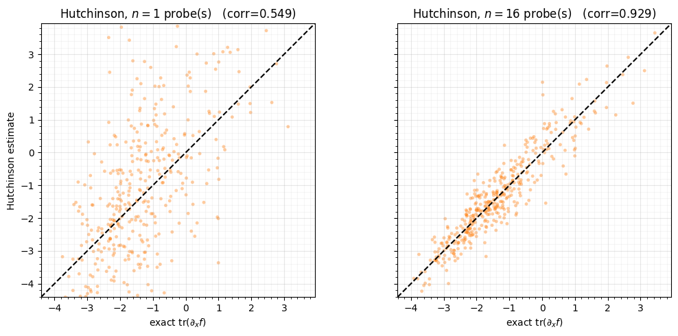

4. The integrated log-determinant¶

Per-step noise is one thing; what we actually train on is the integrated log-det over the whole ODE. The trace estimate enters the augmented dynamics at every solver step, so the errors integrate. We hold the trained vector field fixed, rebuild FFJORD in exact mode (the reference) and in hutchinson mode at several probe counts, and measure the error of $\log p_\theta(x)$ on a held-out batch — the proper version of the quick check from notebook 00. Each FFJORD fixes one probe set, so we average the error over several independent probe draws: the curve then traces the estimator’s behaviour rather than one lucky (or unlucky) draw.

eval_pts = X[:100]
exact_flow = gf.FFJORD(
    jr.key(0), shape=(D,), vector_field=vf, control_dim=0,
    divergence_mode="exact", solver="tsit5", adjoint="direct", rtol=1e-6, atol=1e-6,
)
exact_lp = jax.vmap(Transformed(Normal(jnp.zeros(D)), exact_flow).log_prob)(eval_pts)


def hutch_errors(n, seed):
    """Per-point log p error vs exact, for one fixed probe set."""
    flow = gf.FFJORD(
        jr.key(seed), shape=(D,), vector_field=vf, control_dim=0,
        divergence_mode="hutchinson", n_hutchinson_samples=n,
        solver="tsit5", adjoint="direct", rtol=1e-5, atol=1e-5,
    )
    lp = jax.vmap(Transformed(Normal(jnp.zeros(D)), flow).log_prob)(eval_pts)
    return lp - exact_lp


ns = np.array([1, 2, 4, 8, 16, 32])
n_realizations = 6
biases, rmses = [], []
print(f"exact mean log p = {float(jnp.mean(exact_lp)):+.4f}  "
      f"(each row averaged over {n_realizations} probe draws)\n")
print(f"{'n_probes':>9s}  {'bias':>9s}  {'RMSE':>9s}")
for i, n in enumerate(ns):
    errs = jnp.stack([hutch_errors(int(n), seed=37 * i + 1000 * s + 1)
                      for s in range(n_realizations)])
    b = float(jnp.mean(errs)); r = float(jnp.sqrt(jnp.mean(errs**2)))
    biases.append(b); rmses.append(r)
    print(f"{int(n):>9d}  {b:>+9.4f}  {r:>9.4f}")

fig, ax = plt.subplots(figsize=(6.4, 4.3))
ax.loglog(ns, rmses, "o-", color=DATA_COLOR, label="RMSE of $\\log p$")
ax.loglog(ns, np.abs(biases), "s--", color=LATENT_COLOR, label="|bias| of $\\log p$")
ax.loglog(ns, rmses[0] / np.sqrt(ns / ns[0]), "k:", alpha=0.6, label=r"$\propto 1/\sqrt{n}$")
ax.set(xlabel="Hutchinson probes $n$", ylabel="error vs exact (100 points)",
       title="Integrated log-det error shrinks as $1/\\sqrt{n}$")
ax.legend()
style_ax(ax)
fig.tight_layout()

exact mean log p = -7.5548  (each row averaged over 6 probe draws)

 n_probes       bias       RMSE

        1    +0.1236     2.2566

        2    -0.0415     0.8920

        4    +0.0728     1.1628

        8    -0.0771     0.7785

       16    -0.0400     0.5187

       32    +0.0247     0.3847

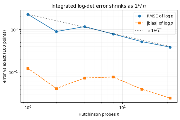
The per-point RMSE follows $1/\sqrt{n}$ , while the bias (the error in the mean log-density) is far smaller — averaging across points cancels the zero-mean per-point noise. So a small probe count gives a trustworthy dataset NLL, but per-point values (anomaly scores, OOD detection) want more probes or the exact trace.

5. Why the probes are fixed per instance¶

A subtle but important choice: gauss_flows draws the Hutchinson probes once at construction (from the FFJORD’s trace_key) and reuses them across every call and every ODE step — the “fixed-noise” variant Grathwohl et al. (2019). The alternative, resampling probes each step, would make $\log p_\theta(x)$ a random function of $x$ , injecting noise into every gradient and destabilising training. Fixing the probes makes the log-det a deterministic function of the parameters, so the optimiser sees a consistent objective. We confirm the determinism.

fixed = gf.FFJORD(jr.key(0), shape=(D,), vector_field=vf, control_dim=0,
                  divergence_mode="hutchinson", n_hutchinson_samples=4,
                  solver="tsit5", adjoint="direct")
x0 = eval_pts[0]
ld_a = float(fixed.transform_and_log_det(x0)[1])
ld_b = float(fixed.transform_and_log_det(x0)[1])
other = gf.FFJORD(jr.key(123), shape=(D,), vector_field=vf, control_dim=0,
                  divergence_mode="hutchinson", n_hutchinson_samples=4,
                  solver="tsit5", adjoint="direct")
ld_c = float(other.transform_and_log_det(x0)[1])
print("same instance, two calls   :", f"{ld_a:+.6f}", "==", f"{ld_b:+.6f}",
      "->", "identical" if ld_a == ld_b else "DIFFER")
print("different trace_key instance:", f"{ld_c:+.6f}",
      "-> differs (a different fixed probe set)")
print("\nFixed probes => log_det is a deterministic function of params => stable gradients.")

same instance, two calls   : -2.140167 == -2.140167 -> identical
different trace_key instance: +1.115355 -> differs (a different fixed probe set)

Fixed probes => log_det is a deterministic function of params => stable gradients.

Calling the same flow twice gives a bit-identical log-det; a flow with a different trace_key gives a different (but still unbiased) value. During training you keep one instance, so the objective is fixed.

6. The cost that makes it worth it — $O(d)$ vs $O(n)$ ¶

The exact trace needs $d$ Jacobian-vector products per ODE step (one per coordinate); Hutchinson needs $n$ , independent of $d$ . As $d$ grows, the exact cost climbs linearly while a fixed-probe Hutchinson stays flat. We time a single divergence evaluation of a DiffeqMLP across dimensions.

def bench(fn, x, reps=25):
    fn(x).block_until_ready()  # warm up / compile
    t0 = time.perf_counter()
    for _ in range(reps):
        fn(x).block_until_ready()
    return (time.perf_counter() - t0) / reps * 1e3  # ms


dims = [2, 8, 32, 128, 512]
t_exact, t_hutch = [], []
for dim in dims:
    vfd = gf.DiffeqMLP(jr.key(dim), in_dim=dim, control_dim=0, hidden=(64, 64))
    xd = jr.normal(jr.key(dim + 1), (dim,))
    f_ex = eqx.filter_jit(lambda x, vfd=vfd: exact_divergence(vfd, 0.5, x, None))
    f_hu = eqx.filter_jit(
        lambda x, vfd=vfd: hutchinson_divergence(vfd, 0.5, x, None, key=jr.key(0), n_samples=1)
    )
    t_exact.append(bench(f_ex, xd))
    t_hutch.append(bench(f_hu, xd))

print(f"{'dim':>6s}  {'exact (ms)':>11s}  {'hutch n=1 (ms)':>15s}  {'JVPs: exact / hutch':>20s}")
for dim, te, th in zip(dims, t_exact, t_hutch):
    print(f"{dim:>6d}  {te:>11.3f}  {th:>15.3f}  {f'{dim} / 1':>20s}")

fig, ax = plt.subplots(figsize=(6.4, 4.3))
ax.loglog(dims, t_exact, "o-", color=DATA_COLOR, label="exact trace ($d$ JVPs)")
ax.loglog(dims, t_hutch, "s-", color=LATENT_COLOR, label="Hutchinson, $n=1$ (1 JVP)")
ax.set(xlabel="dimension $d$", ylabel="time per divergence eval (ms)",
       title="Exact trace grows with $d$; Hutchinson is flat")
ax.legend()
style_ax(ax)
fig.tight_layout()

   dim   exact (ms)   hutch n=1 (ms)   JVPs: exact / hutch
     2        0.243            0.183                 2 / 1
     8        0.324            0.226                 8 / 1
    32        0.233            0.221                32 / 1
   128        0.578            0.259               128 / 1
   512        3.430            0.215               512 / 1

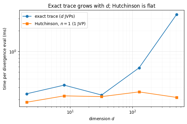
Exact divergence climbs with $d$ (its $d$ JVPs show up as a rising line); the single-probe estimate stays roughly flat. The lines cross at small $d$ — which is exactly why notebook 00 used the exact trace in 2-D and this notebook matters for everything bigger. For image-scale $d\sim10^3$ –10⁶, the exact trace is simply not an option and Hutchinson is the only way the log-det is computable at all.

Recap¶

	exact trace	Hutchinson estimator
cost / ODE step	$O(d)$ JVPs	$O(n)$ JVPs, $n$ fixed
error	none	unbiased, RMSE $\propto 1/\sqrt{n}$
best probe	—	Rademacher (diagonal variance-free)
probes	—	fixed per instance → deterministic log-det
use when	small $d$ / validation	large $d$ / training

Hutchinson is the hinge that turns the elegant trace integral of notebook 00 into a method that runs on images and high-dimensional fields: trade a little variance for an $O(1)$ -per-step log-det, pick Rademacher probes, fix them so training is stable.

Next up. Not every continuous flow needs a stochastic trace. 02 — Matrix-exponential neural flow takes a linear ODE $\dot x = Ax$ , whose flow map is $\exp(At)$ and whose log-det is the exact, closed-form $t\,\operatorname{tr}(A)$ — no estimator, no integration.

References¶

Hutchinson, M. F. (1990). A stochastic estimator of the trace of the influence matrix for Laplacian smoothing splines. Communications in Statistics — Simulation and Computation, 19(2), 433–450.
Grathwohl, W., Chen, R. T. Q., Bettencourt, J., Sutskever, I., & Duvenaud, D. (2019). FFJORD: Free-Form Continuous Dynamics for Scalable Reversible Generative Models. International Conference on Learning Representations (ICLR).