Latent ODE on spirals - Research Notebook

03 — Latent ODE on spirals¶

Notebooks 00-02 Gaussianized with bijections: a deterministic, invertible map carries each data point to $\mathcal{N}(0,I)$ and back, with an exact (or estimated) log-det. That contract breaks the moment the data is a variable-length, irregularly-sampled trajectory — there is no fixed-dimensional $x$ to invert. The latent ODE (Rubanova, Chen & Duvenaud Rubanova et al. (2019), Kidger (2021)) Gaussianizes such data a different way:

Encode the whole trajectory $\{(t_i, x_i)\}$ to a single latent code with a neural-ODE encoder, producing $q(z_0\mid x_{1:N}) = \mathcal{N}(\mu, \sigma^2)$ .
Gaussianize the code by pulling $q(z_0)$ toward the prior $\mathcal{N}(0,I)$ through the ELBO’s KL term — targeting a standard-normal latent (how close it actually gets is itself instructive; see §6).
Evolve $z(t)$ with a second neural ODE $\dot z = f_\theta(z,t)$ and decode $z(t_i)\mapsto \hat x_i$ .

This is a stochastic Gaussianizer, not a bijection — the SurVAE-style cousin (Part 8) of the flows above. It trades exact invertibility for two things the bijections cannot do: ingest irregular sequences of any length, and change dimension ( $\mathbb{R}^{N\times 2}\to\mathbb{R}^{d_z}$ ). The ODE prior also makes extrapolation natural — integrate $z(t)$ past the last observation. It is the bridge from Part 6 to the time-series Gaussianization of Part 11.

What you will see

Toy spirals, densely defined but irregularly observed (the realistic setting).
The encode → latent-ODE → decode VAE, trained by ELBO with gf.DiffeqMLP fields.
Reconstruction of held-out spirals from a handful of irregular points.
Extrapolation beyond the observed window by integrating the latent ODE forward.
The latent Gaussianization — and the topological obstruction (a circular phase cannot be pushed into a Euclidean Gaussian) that keeps it only approximate.

import warnings

warnings.filterwarnings("ignore")

import diffrax
import equinox as eqx
import interpax
import jax
import jax.nn as jnn
import jax.numpy as jnp
import jax.random as jr
import matplotlib.pyplot as plt
import numpy as np
import optax
from scipy import stats

from gauss_flows import DiffeqMLP, pack_time_control
from _style import DATA_COLOR, GAUSS_KW, LATENT_COLOR, SCATTER_KW, style_ax

jax.config.update("jax_enable_x64", True)

1. Irregularly-sampled spiral dataset¶

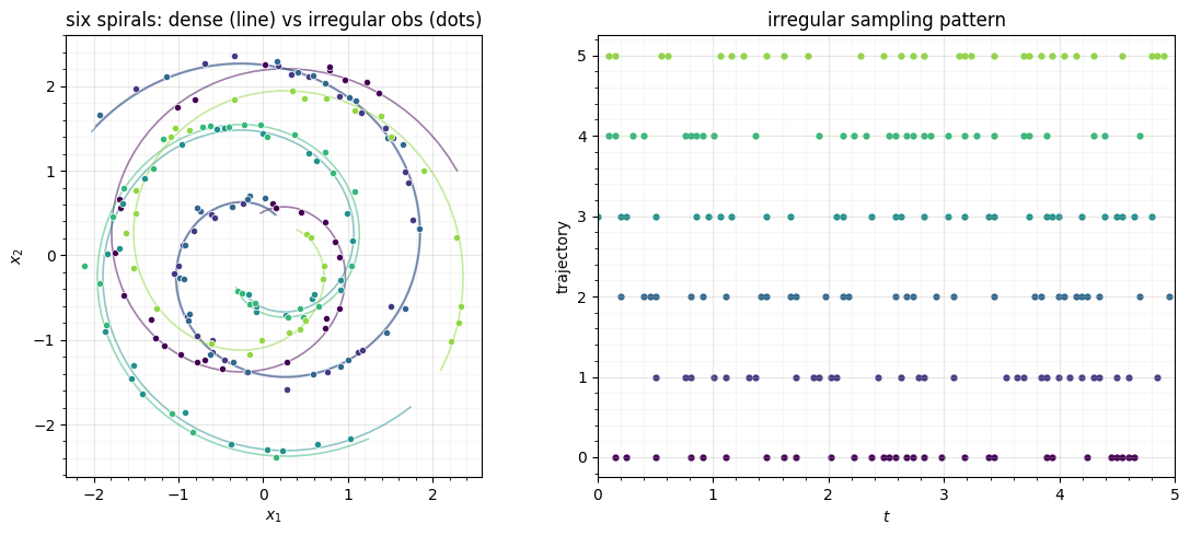
Following Rubanova et al. §4.1: 2-D spirals with a random phase and a random direction (clockwise / counter-clockwise), defined densely on a common grid but then irregularly subsampled with additive noise — the situation real sensors produce. A held-out split backs the reconstruction and extrapolation figures.

N_TRAJ, N_EVAL = 250, 50
T_MAX, N_DENSE, N_OBS, NOISE_STD = 5.0, 100, 30, 0.05


def _spiral(key, t):
    rot_key, dir_key = jr.split(key)
    theta = jr.uniform(rot_key, minval=0.0, maxval=2 * jnp.pi)
    direction = jr.choice(dir_key, jnp.array([-1.0, 1.0]))
    r = 0.4 * t + 0.5
    angle = direction * (1.5 * t) + theta
    return jnp.stack([r * jnp.cos(angle), r * jnp.sin(angle)], axis=-1)


def make_dataset(key, n_traj):
    spiral_key, sample_key, noise_key = jr.split(key, 3)
    t_dense = jnp.linspace(0.0, T_MAX, N_DENSE)

    def per_traj(sk, mk):
        x_clean = _spiral(sk, t_dense)
        idx = jnp.sort(jr.choice(mk, N_DENSE, shape=(N_OBS,), replace=False))
        return x_clean, t_dense[idx], x_clean[idx]

    x_clean, t_obs, x_obs_clean = jax.vmap(per_traj)(
        jr.split(spiral_key, n_traj), jr.split(sample_key, n_traj)
    )
    x_obs = x_obs_clean + NOISE_STD * jr.normal(noise_key, x_obs_clean.shape)
    return t_dense, x_clean, t_obs, x_obs


t_dense, x_clean, t_obs, x_obs = make_dataset(jr.key(0), N_TRAJ)
n_train = N_TRAJ - N_EVAL
t_obs_tr, t_obs_ev = t_obs[:n_train], t_obs[n_train:]
x_obs_tr, x_obs_ev = x_obs[:n_train], x_obs[n_train:]
x_clean_ev = x_clean[n_train:]
print(f"{N_TRAJ} spirals ({n_train} train / {N_EVAL} eval), "
      f"{N_OBS} irregular obs each on t in [0, {T_MAX}]")

fig, (ax_xy, ax_t) = plt.subplots(1, 2, figsize=(11.5, 5))
for k in range(6):
    c = plt.cm.viridis(k / 6)
    ax_xy.plot(np.asarray(x_clean[k, :, 0]), np.asarray(x_clean[k, :, 1]), color=c, alpha=0.5, lw=1.2)
    ax_xy.scatter(np.asarray(x_obs[k, :, 0]), np.asarray(x_obs[k, :, 1]), s=20, color=c,
                  edgecolor="white", linewidth=0.5, zorder=3)
    ax_t.scatter(np.asarray(t_obs[k]), np.full(N_OBS, k), s=12, color=c)
ax_xy.set(title="six spirals: dense (line) vs irregular obs (dots)", xlabel="$x_1$", ylabel="$x_2$")
ax_xy.set_aspect("equal"); style_ax(ax_xy)
ax_t.set(title="irregular sampling pattern", xlabel="$t$", ylabel="trajectory", xlim=(0, T_MAX))
style_ax(ax_t)
fig.tight_layout()

250 spirals (200 train / 50 eval), 30 irregular obs each on t in [0, 5.0]

2. The model: encode → latent ODE → decode¶

Three small modules, both vector fields being gf.DiffeqMLP. The encoder runs a forward neural ODE on the linearly-interpolated observation path $\hat X(t)$ — the observations enter as the control of the time-control condition, so the same DiffeqMLP plumbing that FFJORD used carries over — and maps the final hidden state to $(\mu, \log\sigma^2)$ of $q(z_0)$ . The dynamics field evolves $z(t)$ ; the decoder is an MLP $z(t_i)\mapsto\hat x_i$ with fixed observation noise.

OBS_DIM, LATENT_DIM, ENC_HIDDEN, DEC_HIDDEN, SIGMA_OBS = 2, 4, 25, 20, 0.20


def _interp(t_query, t_traj, x_traj):
    return interpax.interp1d(jnp.atleast_1d(t_query), t_traj, x_traj, method="linear", extrap=True)[0]


def _solve(vf, y0, t0, t1, args=None, saveat=None):
    return diffrax.diffeqsolve(
        diffrax.ODETerm(vf), diffrax.Tsit5(), t0=t0, t1=t1, dt0=0.05, y0=y0, args=args,
        saveat=saveat or diffrax.SaveAt(t1=True),
        stepsize_controller=diffrax.PIDController(rtol=1e-3, atol=1e-4),
        adjoint=diffrax.RecursiveCheckpointAdjoint(), max_steps=4096,
    )


class LatentODE(eqx.Module):
    encoder_vf: DiffeqMLP
    enc_head: eqx.nn.Linear
    dynamics_vf: DiffeqMLP
    decoder: eqx.nn.MLP

    def __init__(self, key):
        ke, kh, kd, kc = jr.split(key, 4)
        self.encoder_vf = DiffeqMLP(ke, in_dim=ENC_HIDDEN, control_dim=OBS_DIM, hidden=(40, 40), activation=jnn.tanh)
        self.enc_head = eqx.nn.Linear(ENC_HIDDEN, 2 * LATENT_DIM, key=kh)
        self.dynamics_vf = DiffeqMLP(kd, in_dim=LATENT_DIM, control_dim=0, hidden=(40, 40), activation=jnn.tanh)
        self.decoder = eqx.nn.MLP(LATENT_DIM, OBS_DIM, DEC_HIDDEN, 2, activation=jnn.tanh, key=kc)

    def encode(self, t_traj, x_traj):
        def vf(t, h, args):
            return self.encoder_vf(t, h, pack_time_control(t, _interp(t, args[0], args[1])))

        h_final = _solve(vf, jnp.zeros(ENC_HIDDEN), t_traj[0], t_traj[-1], args=(t_traj, x_traj)).ys[-1]
        mu, log_var = jnp.split(self.enc_head(h_final), 2)
        return mu, jnp.clip(log_var, -8.0, 4.0)

    def decode(self, z0, times):
        z_traj = _solve(lambda t, z, a: self.dynamics_vf(t, z, None), z0, times[0], times[-1],
                        saveat=diffrax.SaveAt(ts=times)).ys
        return jax.vmap(self.decoder)(z_traj)

    def elbo(self, key, t_traj, x_traj):
        mu, log_var = self.encode(t_traj, x_traj)
        z0 = mu + jnp.exp(0.5 * log_var) * jr.normal(key, mu.shape)
        x_hat = self.decode(z0, t_traj)
        recon = jnp.sum(-0.5 * ((x_traj - x_hat) / SIGMA_OBS) ** 2 - jnp.log(SIGMA_OBS) - 0.5 * jnp.log(2 * jnp.pi))
        kl = 0.5 * jnp.sum(jnp.exp(log_var) + mu**2 - 1.0 - log_var)
        return recon - kl, recon, kl


model_key, train_key, eval_key = jr.split(jr.key(0), 3)
model = LatentODE(model_key)
n_params = sum(int(np.prod(p.shape)) for p in jax.tree_util.tree_leaves(eqx.filter(model, eqx.is_array)))
print(f"latent dim {LATENT_DIM}, encoder hidden {ENC_HIDDEN}, obs noise {SIGMA_OBS}")
print(f"trainable parameters: {n_params}")

latent dim 4, encoder hidden 25, obs noise 0.2
trainable parameters: 6679

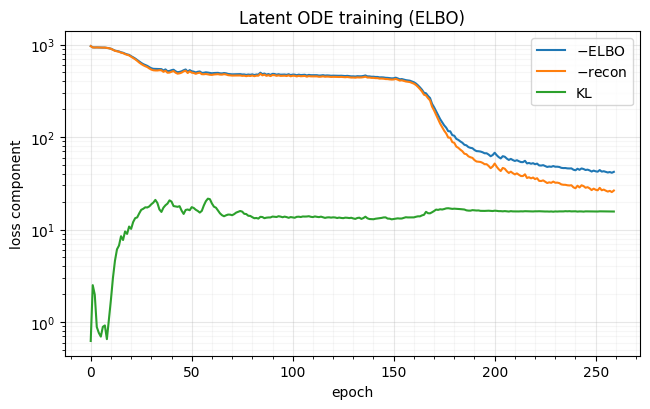
3. Train by the ELBO¶

Each step encodes every trajectory with one forward ODE solve, samples $z_0$ by the reparametrisation trick, decodes with a second ODE solve at the observed times, and adds the Gaussian log-likelihood to the closed-form KL. Two ODE solves per trajectory make this the heaviest cell in Part 6; a cosine learning-rate decay lets it settle inside a short budget.

N_EPOCHS, BATCH = 260, 50
n_batches = n_train // BATCH
lr = optax.cosine_decay_schedule(3e-3, decay_steps=N_EPOCHS * n_batches, alpha=0.02)
optimizer = optax.chain(optax.clip_by_global_norm(5.0), optax.adam(lr))
opt_state = optimizer.init(eqx.filter(model, eqx.is_array))


@eqx.filter_jit
def loss_fn(model, key, t_b, x_b):
    keys = jr.split(key, t_b.shape[0])
    e, r, k = jax.vmap(model.elbo)(keys, t_b, x_b)
    return -jnp.mean(e), (jnp.mean(r), jnp.mean(k))


@eqx.filter_jit
def step(model, opt_state, key, t_b, x_b):
    (loss, (recon, kl)), grads = eqx.filter_value_and_grad(loss_fn, has_aux=True)(model, key, t_b, x_b)
    updates, opt_state = optimizer.update(grads, opt_state, model)
    return eqx.apply_updates(model, updates), opt_state, loss, recon, kl


losses, recons, kls = [], [], []
for epoch in range(N_EPOCHS):
    train_key, perm_key, batch_key = jr.split(train_key, 3)
    perm = jr.permutation(perm_key, n_train)
    t_sh, x_sh = t_obs_tr[perm], x_obs_tr[perm]
    el, er, ek = 0.0, 0.0, 0.0
    for b in range(n_batches):
        sl = slice(b * BATCH, (b + 1) * BATCH)
        batch_key, sub = jr.split(batch_key)
        model, opt_state, loss, recon, kl = step(model, opt_state, sub, t_sh[sl], x_sh[sl])
        el += float(loss); er += float(recon); ek += float(kl)
    losses.append(el / n_batches); recons.append(er / n_batches); kls.append(ek / n_batches)
    if epoch == 0 or (epoch + 1) % 40 == 0:
        print(f"epoch {epoch + 1:>4d}  -ELBO {losses[-1]:>9.2f}  -recon {-recons[-1]:>9.2f}  KL {kls[-1]:>6.2f}")

fig, ax = plt.subplots(figsize=(6.6, 4.2))
ep = np.arange(len(losses))
ax.plot(ep, losses, color=DATA_COLOR, label="$-$ELBO")
ax.plot(ep, [-r for r in recons], color=LATENT_COLOR, label="$-$recon")
ax.plot(ep, kls, color="tab:green", label="KL")
ax.set(xlabel="epoch", ylabel="loss component", title="Latent ODE training (ELBO)", yscale="log")
ax.legend()
style_ax(ax)
fig.tight_layout()

epoch    1  -ELBO    964.21  -recon    963.58  KL   0.62

epoch   40  -ELBO    519.39  -recon    498.69  KL  20.70

epoch   80  -ELBO    471.89  -recon    457.85  KL  14.04

epoch  120  -ELBO    460.54  -recon    447.08  KL  13.47

epoch  160  -ELBO    399.27  -recon    385.68  KL  13.59

epoch  200  -ELBO     63.93  -recon     48.07  KL  15.86

epoch  240  -ELBO     44.38  -recon     28.63  KL  15.76

4. Reconstruction from irregular observations¶

For each held-out spiral we encode its handful of irregular, noisy points, then decode on the dense grid. The latent ODE produces a smooth curve that threads the observations — interpolation in continuous time, learned from the trajectory family.

@eqx.filter_jit
def reconstruct(model, key, t_traj, x_traj, t_target):
    mu, log_var = model.encode(t_traj, x_traj)
    z0 = mu + jnp.exp(0.5 * log_var) * jr.normal(key, mu.shape)
    return model.decode(z0, t_target)


rec_keys = jr.split(eval_key, 6)
fig, axes = plt.subplots(2, 3, figsize=(14, 8.5))
for k, ax in enumerate(axes.flat):
    x_hat = reconstruct(model, rec_keys[k], t_obs_ev[k], x_obs_ev[k], t_dense)
    ax.plot(np.asarray(x_clean_ev[k, :, 0]), np.asarray(x_clean_ev[k, :, 1]), color="0.4", lw=1.0, label="ground truth")
    ax.plot(np.asarray(x_hat[:, 0]), np.asarray(x_hat[:, 1]), color=DATA_COLOR, lw=2.0, label="reconstruction")
    ax.scatter(np.asarray(x_obs_ev[k, :, 0]), np.asarray(x_obs_ev[k, :, 1]), s=20, color=LATENT_COLOR,
               edgecolor="white", linewidth=0.5, zorder=3, label="observations")
    ax.set(title=f"held-out spiral {k}", xlabel="$x_1$", ylabel="$x_2$")
    ax.set_aspect("equal"); style_ax(ax)
    if k == 0:
        ax.legend(loc="upper left", framealpha=0.9, fontsize=9)
fig.tight_layout()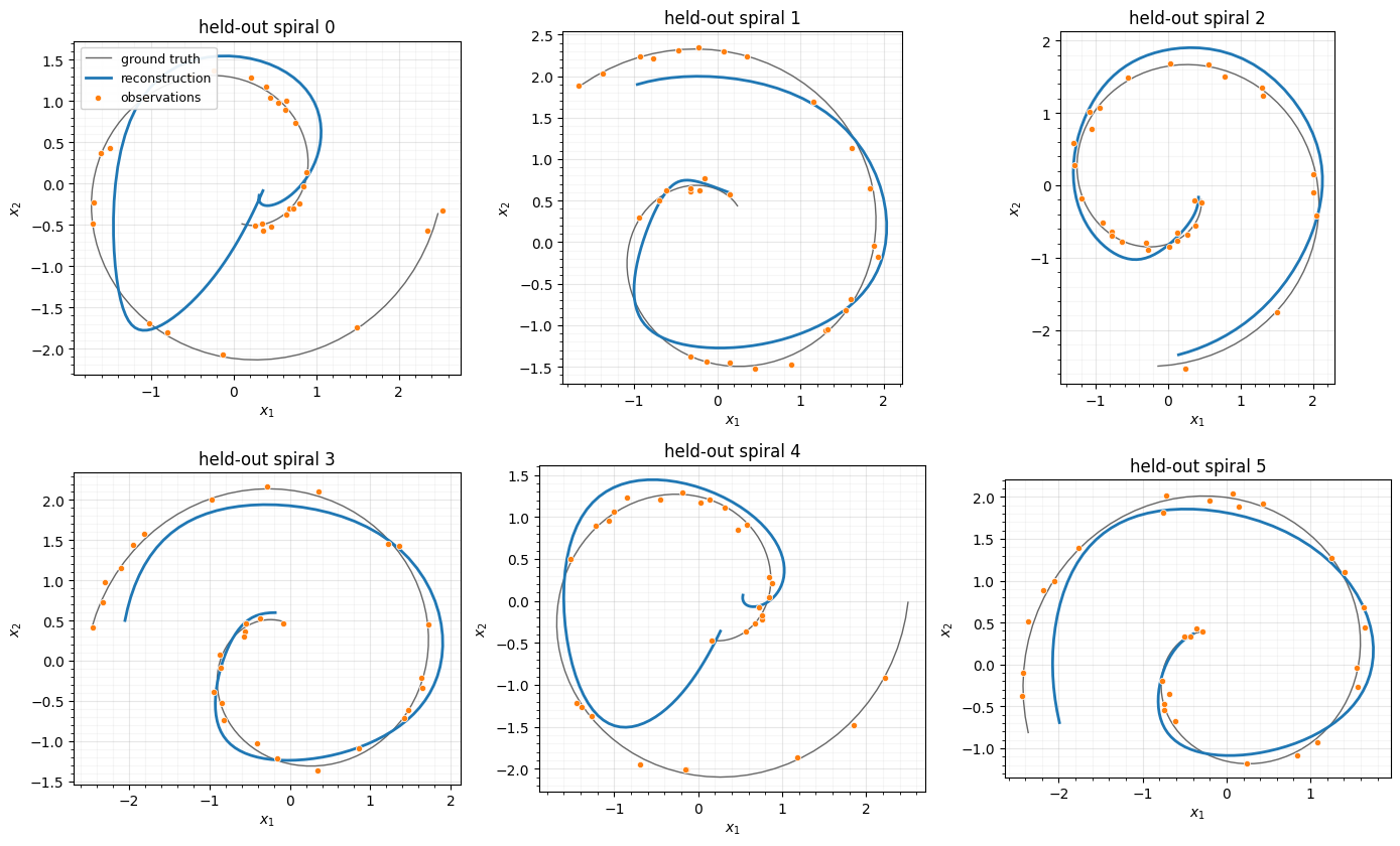

5. Extrapolation past the observed window¶

Because the latent prior is an ODE, the model extrapolates for free: encode using only the observations on $[0, T/2]$ , then integrate $z(t)$ all the way to $T$ . The dashed arm is pure forward prediction — the model never saw those times for this trajectory.

T_HALF = T_MAX / 2.0
fig, axes = plt.subplots(2, 3, figsize=(14, 8.5))
for k, ax in enumerate(axes.flat):
    mask = t_obs_ev[k] <= T_HALF
    n_keep = int(jnp.sum(mask))
    if n_keep < 4:
        ax.set_visible(False); continue
    t_half, x_half = t_obs_ev[k][:n_keep], x_obs_ev[k][:n_keep]
    mu, _ = model.encode(t_half, x_half)
    x_hat = model.decode(mu, t_dense)  # posterior mean for a clean curve
    dense_obs = np.asarray(t_dense <= T_HALF)
    ax.plot(np.asarray(x_clean_ev[k, :, 0]), np.asarray(x_clean_ev[k, :, 1]), color="0.4", lw=1.0, label="ground truth")
    ax.plot(np.asarray(x_hat[dense_obs, 0]), np.asarray(x_hat[dense_obs, 1]), color=DATA_COLOR, lw=2.0, label=r"recon ($t\leq T/2$)")
    ax.plot(np.asarray(x_hat[~dense_obs, 0]), np.asarray(x_hat[~dense_obs, 1]), color="tab:red", lw=2.0, ls="--", label=r"extrapolation ($t>T/2$)")
    ax.scatter(np.asarray(x_half[:, 0]), np.asarray(x_half[:, 1]), s=20, color=LATENT_COLOR, edgecolor="white", linewidth=0.5, zorder=3)
    ax.set(title=f"held-out spiral {k}", xlabel="$x_1$", ylabel="$x_2$")
    ax.set_aspect("equal"); style_ax(ax)
    if k == 0:
        ax.legend(loc="upper left", framealpha=0.9, fontsize=9)
fig.tight_layout()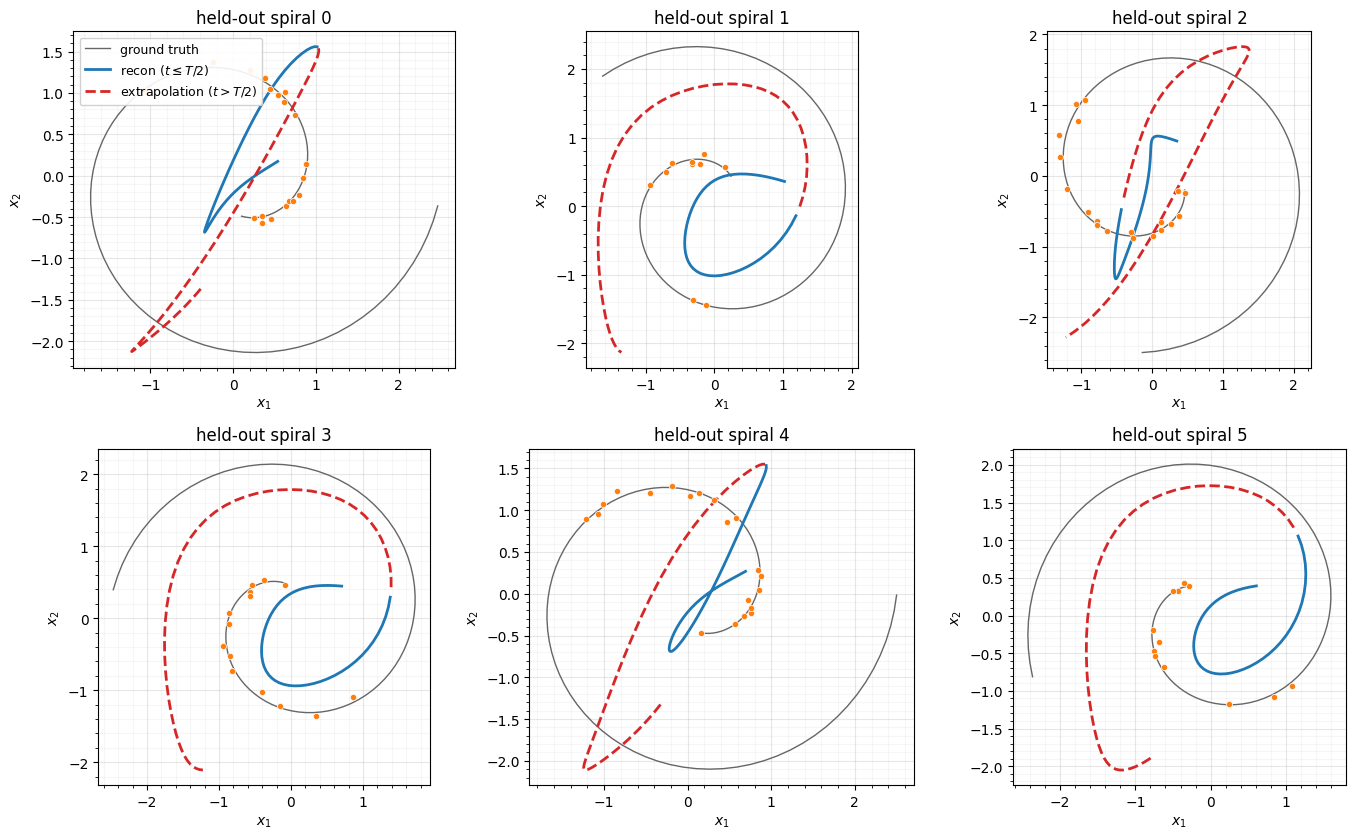

6. The Gaussianization check — the latent code¶

Now the Gaussianization question for the whole part: how standard-normal is the latent? The ELBO’s KL pulls each $q(z_0\mid x)$ toward the prior, so we plot the aggregate posterior — the encoded $z_0$ across the dataset — against $\mathcal{N}(0,I)$ and read off its moments.

mus = jax.vmap(lambda t, x: model.encode(t, x)[0])(t_obs, x_obs)  # posterior means, (N_TRAJ, LATENT_DIM)
mus = np.asarray(mus)

fig, axes = plt.subplots(1, 3, figsize=(15, 4.6))
ax = axes[0]
ax.scatter(mus[:, 0], mus[:, 1], color=LATENT_COLOR, **SCATTER_KW)
th = np.linspace(0, 2 * np.pi, 200)
for r in (1.0, 2.0):
    ax.plot(r * np.cos(th), r * np.sin(th), **GAUSS_KW)
ax.set(title=r"latent codes $z_0$ (dims 0, 1)", xlabel="$z_0^{(0)}$", ylabel="$z_0^{(1)}$",
       xlim=(-3.4, 3.4), ylim=(-3.4, 3.4))
ax.set_aspect("equal"); style_ax(ax)
for j, ax in enumerate(axes[1:]):
    osm, osr = stats.probplot(mus[:, j], dist="norm", fit=False)
    ax.scatter(osm, osr, color=LATENT_COLOR, s=8, alpha=0.5, edgecolors="none")
    ax.plot([-3.4, 3.4], [-3.4, 3.4], **GAUSS_KW)
    ax.set(title=f"QQ plot — $z_0^{{({j})}}$", xlabel="theoretical", ylabel="empirical",
           xlim=(-3.4, 3.4), ylim=(-3.4, 3.4))
    ax.set_aspect("equal"); style_ax(ax)
fig.tight_layout()

print(f"mean KL(q(z0) || N(0,I)) over dataset: {np.mean(kls[-1]):.3f}  (final-epoch batch mean)")
print("aggregate latent moments (target 0, 1, 0, 0):")
for j in range(LATENT_DIM):
    z = mus[:, j]
    print(f"  z0[{j}]: mean={z.mean():+.3f}  std={z.std():.3f}  skew={stats.skew(z):+.3f}  exc-kurt={stats.kurtosis(z):+.3f}")

mean KL(q(z0) || N(0,I)) over dataset: 15.674  (final-epoch batch mean)
aggregate latent moments (target 0, 1, 0, 0):
  z0[0]: mean=+1.324  std=1.491  skew=+0.203  exc-kurt=-0.715
  z0[1]: mean=-1.270  std=0.995  skew=-0.105  exc-kurt=-1.654
  z0[2]: mean=-1.117  std=1.028  skew=+0.057  exc-kurt=-0.786
  z0[3]: mean=+0.510  std=1.150  skew=-0.296  exc-kurt=-0.490

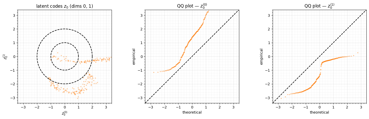
The KL did its job in part — the codes are roughly centred and unit-scale, not the runaway spread an unregularised autoencoder would give — but they are plainly not $\mathcal{N}(0,I)$ : the scatter shows arc-like clusters, the QQ plots bend off the diagonal, and the strongly negative excess kurtosis is the fingerprint of a ring / bimodal distribution rather than a Gaussian. That is not just the usual VAE aggregate-posterior gap; it is a topological obstruction. The spiral family is indexed by a circular phase and a binary direction, and neither a circle nor two discrete modes can be pushed smoothly into a Euclidean $\mathcal{N}(0,I)$ — the same wall the bijective flows of Parts 0-5 hit on periodic data.

This is the honest limit of stochastic Gaussianization, and it points three ways: to Part 8 (surjections / stochastic transforms that formalise this lossy encode-decode), to Part 10 (non-Euclidean Gaussianization — the right target geometry for a circular latent), and to Part 19 (replacing the fixed $\mathcal{N}(0,I)$ prior with a learned flow prior that can absorb such structure). What the latent ODE delivers regardless is the practical payoff above: a single code, learned through a standard-normal prior, from which the ODE reconstructs and extrapolates irregular trajectories.

Recap — and the end of Part 6¶

	bijective CNF (00-02)	latent ODE (here)
maps	data point $\leftrightarrow \mathcal{N}(0,I)$	whole trajectory $\to$ code $z_0$
invertible	yes, exactly	no — stochastic encode/decode (ELBO)
log-det	trace integral / $t\,\operatorname{tr}(W)$	n/a — KL to the prior instead
dimension	preserved	changed ( $\mathbb{R}^{N\times 2}\to\mathbb{R}^{d_z}$ )
handles	fixed- $d$ vectors	irregular, variable-length sequences

Part 6 walked the continuous-time family from one end to the other: the free-form FFJORD with its trace-integral log-det (00), the Hutchinson estimator that makes that trace scale (01), the closed-form matrix-exponential linear flow (02), and now the latent ODE, which gives up bijectivity to Gaussianize structured, irregular trajectories into a latent code. The first three are continuous bijections; this last is a continuous stochastic transform — the hinge to Part 8 (SurVAE surjections & stochastic flows).

Where this goes next. The latent ODE is the template for Part 11 (time-series Gaussianization — autoregressive and latent-ODE models for sequences) and feeds the probabilistic-programming integrations of Part 19 (flows and latent-variable models as priors/guides). Part 6 is complete.

References¶

Rubanova, Y., Chen, R. T. Q., & Duvenaud, D. (2019). Latent Ordinary Differential Equations for Irregularly-Sampled Time Series. Advances in Neural Information Processing Systems (NeurIPS).
Kidger, P. (2021). On Neural Differential Equations [Phdthesis]. University of Oxford.