Matrix-exponential neural flow

02 — Matrix-exponential neural flow¶

Notebooks 00 and 01 paid two prices for a free-form continuous flow: an ODE solve in both directions, and a stochastic estimate of the log-det trace. Both prices vanish the moment the vector field is linear. Take

\frac{\mathrm{d}x_t}{\mathrm{d}t} = W x_t \;\;\Longrightarrow\;\; x_t = \exp(W t)\,x_0,

((1))

the matrix exponential. The instantaneous change-of-variables trace is now constant in $x$ — $\operatorname{tr}(\partial_x (Wx)) = \operatorname{tr}(W)$ — so the log-det integral collapses to a closed form:

\log\big|\det \partial x_T/\partial x_0\big| = \int_0^T \operatorname{tr}(W)\,\mathrm{d}t = T\,\operatorname{tr}(W).

((2))

gauss_flows.MatrixExponential adds a time-gated bias, $y = \exp(W t)\,x + h(t)\,b$ , and is a neural flow Biloš et al. (2021), Kidger (2021): the closed-form solution of an ODE rather than something a solver integrates. It is the continuous-time face of Part 2’s linear mixers — a trainable, exactly-invertible rotation-plus-scale with a free, analytic log-det. The catch is the flip side of the gift: a linear map is affine, so on its own it can only Gaussianize a Gaussian.

What you will see

A single layer morphing a ring as $t:0\to1$ — the identity at $t=0$ since $\exp(0)=I$ .
The log-det is exactly $t\,\operatorname{tr}(W)$ — checked against autodiff slogdet.
It Gaussianizes an anisotropic Gaussian exactly (latent $\to\mathcal{N}(0,I)$ ).
It cannot Gaussianize two moons — the affine ceiling, and why you compose it with nonlinear blocks (Parts 4-5) or use FFJORD.
The $t$ -indexed family of distributions a single trained model encodes for free.

import warnings

warnings.filterwarnings("ignore")

import equinox as eqx
import jax
import jax.numpy as jnp
import jax.random as jr
import matplotlib.pyplot as plt
import numpy as np
import optax
from flowjax.bijections import Chain
from flowjax.distributions import Normal, Transformed
from flowjax.train import fit_to_data
from scipy import stats
from sklearn.datasets import make_moons

from gauss_flows import MatrixExponential, TimeTanh, pack_time_control
from _style import DATA_COLOR, GAUSS_KW, LATENT_COLOR, SCATTER_KW, style_ax

jax.config.update("jax_enable_x64", True)

1. A single layer morphing a ring¶

Push the unit circle through $\exp(W t)\,\cdot + h(t)\,b$ for $t\in[0,1]$ . At $t=0$ the map is the identity ( $\exp(0)=I$ , $h(0)=0$ ), and as $t$ grows it becomes a rotated, scaled, shifted ellipse — a continuum of affine maps indexed by $t$ .

single = MatrixExponential(jr.key(0), shape=(2,), w_init_scale=0.6)
th = jnp.linspace(0.0, 2 * jnp.pi, 200)
ring = jnp.stack([jnp.cos(th), jnp.sin(th)], axis=-1)

times = jnp.linspace(0.0, 1.0, 5)
fig, axes = plt.subplots(1, 5, figsize=(16, 3.6), sharex=True, sharey=True)
for ax, t in zip(axes, times):
    pushed = jax.vmap(lambda p: single.transform_and_log_det(p, pack_time_control(float(t)))[0])(ring)
    ax.plot(np.asarray(ring[:, 0]), np.asarray(ring[:, 1]), color="0.6", lw=1.0)
    ax.plot(np.asarray(pushed[:, 0]), np.asarray(pushed[:, 1]), color=DATA_COLOR, lw=2.0)
    ax.set(title=rf"$t={float(t):.2f}$", xlabel="$x_1$", xlim=(-2.5, 2.5), ylim=(-2.5, 2.5))
    ax.set_aspect("equal")
    style_ax(ax)
axes[0].set_ylabel("$x_2$")
fig.suptitle(r"A single $\exp(Wt)$ layer: identity at $t=0$, affine warp by $t=1$", y=1.04)
fig.tight_layout()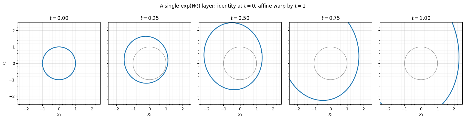

2. The log-det is exactly $t\,\operatorname{tr}(W)$ ¶

This is the whole appeal: no trace integral to estimate, no solver — the log-det is the analytic $t\,\operatorname{tr}(W)$ , independent of the bias gate $h$ (a shift never scales volume). We check it against an autodiff slogdet of the Jacobian on a 4-D layer with a learned time gate, across a range of query times.

gate_key, w_key = jr.split(jr.key(1))
checked = MatrixExponential(w_key, shape=(4,), time_bias_net=TimeTanh(gate_key, embedding_dim=8),
                            w_init_scale=0.2)
x_eval = jr.normal(jr.key(2), (4,))
ts = jnp.linspace(-1.0, 1.0, 21)


def forward(x, t):
    return checked.transform_and_log_det(x, pack_time_control(t))[0]


closed = jax.vmap(lambda t: t * jnp.trace(checked.W))(ts)
ad = jax.vmap(lambda t: jnp.linalg.slogdet(jax.jacrev(forward)(x_eval, t))[1])(ts)

fig, ax = plt.subplots(figsize=(6.2, 4.2))
ax.plot(np.asarray(ts), np.asarray(ad), "o", color=LATENT_COLOR, ms=8,
        label=r"autodiff $\log|\det\,\partial y/\partial x|$")
ax.plot(np.asarray(ts), np.asarray(closed), "-", color=DATA_COLOR, lw=2,
        label=r"closed-form $t\,\mathrm{tr}(W)$")
ax.set(xlabel="$t$", ylabel=r"$\log|\det\,\partial y/\partial x|$",
       title="Closed-form log-det matches autodiff")
ax.legend()
style_ax(ax)
fig.tight_layout()
print(f"max |closed-form - autodiff| over 21 times: {float(jnp.max(jnp.abs(closed - ad))):.2e}")

max |closed-form - autodiff| over 21 times: 4.72e-16

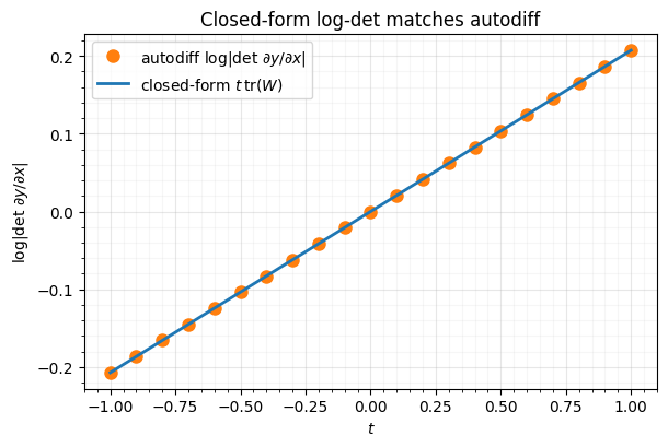
Agreement to machine precision. The log-det never touches the Jacobian — it reads $\operatorname{tr}(W)$ straight off the weight matrix.

3. Gaussianizing an anisotropic Gaussian — exactly¶

A linear flow is exactly the right tool when the data is Gaussian: whitening a correlated, tilted Gaussian to $\mathcal{N}(0,I)$ is a linear map, and MatrixExponential represents it with a closed-form log-det. We fit a short chain (each block its own $W$ , $b$ , gate) to a tilted anisotropic Gaussian, querying the time at $t=1$ so the chain acts as a fixed composition.

angle = jnp.pi / 6
R = jnp.array([[jnp.cos(angle), -jnp.sin(angle)], [jnp.sin(angle), jnp.cos(angle)]])
gauss = (jr.normal(jr.key(7), (2000, 2)) * jnp.array([1.7, 0.7])) @ R.T + jnp.array([0.5, -0.5])


def make_chain(key, n_layers=3):
    keys = jr.split(key, n_layers)
    return Chain([
        MatrixExponential(k, shape=(2,), time_bias_net=TimeTanh(jr.fold_in(k, 99), embedding_dim=8),
                          w_init_scale=0.3)
        for k in keys
    ])


def fit_chain(key, data, n_layers=3, max_epochs=250):
    # Closed-form flow => training is cheap; run a cosine-decayed schedule to
    # convergence (no early stopping) so the linear whitening actually settles.
    dist = Transformed(Normal(jnp.zeros(2)), make_chain(key, n_layers))
    t_one = jnp.broadcast_to(pack_time_control(1.0), (data.shape[0], 1))
    steps = -(-int(data.shape[0] * 0.9) // 256)
    sched = optax.cosine_decay_schedule(5e-3, decay_steps=max_epochs * steps, alpha=0.01)
    opt = optax.chain(optax.clip_by_global_norm(5.0), optax.adam(sched))
    trained, losses = fit_to_data(key, dist, (data, t_one), optimizer=opt,
                                  max_epochs=max_epochs, max_patience=max_epochs,
                                  batch_size=256, val_prop=0.1, show_progress=False)
    return trained, losses


gauss_dist, gauss_losses = fit_chain(jr.key(0), gauss)
print(f"anisotropic-Gaussian fit: stopped at {len(gauss_losses['train'])} epochs, "
      f"val NLL = {float(min(gauss_losses['val'])):.4f}")

anisotropic-Gaussian fit: stopped at 250 epochs, val NLL = 3.0454

def gaussianize(chain, data):
    c1 = pack_time_control(1.0)
    return np.asarray(jax.vmap(lambda x: chain.inverse_and_log_det(x, c1)[0])(data))


def density_grid(dist, lim=3.5, n=80):
    xs = jnp.linspace(-lim, lim, n)
    gx, gy = jnp.meshgrid(xs, xs)
    pts = jnp.stack([gx.ravel(), gy.ravel()], -1)
    cond = jnp.broadcast_to(pack_time_control(1.0), (pts.shape[0], 1))
    lp = eqx.filter_jit(lambda p, c: jax.vmap(dist.log_prob)(p, c))(pts, cond)
    return gx, gy, jnp.exp(lp).reshape(n, n)


gx, gy, dens = density_grid(gauss_dist)
samp = gauss_dist.sample(jr.key(5), (2000,), condition=pack_time_control(1.0))

fig, (ax_d, ax_s) = plt.subplots(1, 2, figsize=(11.5, 5))
ax_d.contourf(np.asarray(gx), np.asarray(gy), np.asarray(dens), levels=20, cmap="viridis")
ax_d.set(title=r"learned density $p_\theta(x)$ (closed-form, $t=1$)", xlabel="$x_1$", ylabel="$x_2$")
ax_d.set_aspect("equal"); style_ax(ax_d)
ax_s.scatter(np.asarray(gauss[:, 0]), np.asarray(gauss[:, 1]), color=DATA_COLOR, label="data", **SCATTER_KW)
ax_s.scatter(np.asarray(samp[:, 0]), np.asarray(samp[:, 1]), color="tab:red", marker="x",
             s=10, alpha=0.4, linewidths=0.7, label="flow samples")
ax_s.set(title="data vs. flow samples", xlabel="$x_1$", ylabel="$x_2$", xlim=(-3.5, 3.5), ylim=(-3.5, 3.5))
ax_s.set_aspect("equal"); ax_s.legend(loc="upper right", framealpha=0.9); style_ax(ax_s)
fig.tight_layout()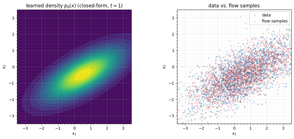

Now the Gaussianization direction: push the data through the inverse map and check the pushforward is standard normal.

Z = gaussianize(gauss_dist.bijection, gauss)
fig, axes = plt.subplots(1, 3, figsize=(15, 4.6))
ax = axes[0]
ax.scatter(Z[:, 0], Z[:, 1], color=LATENT_COLOR, **SCATTER_KW)
for r in (1.0, 2.0):
    ax.plot(r * np.cos(th), r * np.sin(th), **GAUSS_KW)
ax.set(title=r"Gaussianized data $z=T^{-1}(x)$", xlabel="$z_1$", ylabel="$z_2$",
       xlim=(-3.6, 3.6), ylim=(-3.6, 3.6))
ax.set_aspect("equal"); style_ax(ax)
for j, ax in enumerate(axes[1:]):
    osm, osr = stats.probplot(Z[:, j], dist="norm", fit=False)
    ax.scatter(osm, osr, color=LATENT_COLOR, s=8, alpha=0.5, edgecolors="none")
    ax.plot([-3.5, 3.5], [-3.5, 3.5], **GAUSS_KW)
    ax.set(title=f"QQ plot — $z_{j + 1}$", xlabel="theoretical", ylabel="empirical",
           xlim=(-3.5, 3.5), ylim=(-3.5, 3.5))
    ax.set_aspect("equal"); style_ax(ax)
fig.tight_layout()
print("Gaussianized moments (target 0, 1, 0, 0):")
for j in range(2):
    z = Z[:, j]
    print(f"  z_{j + 1}: mean={z.mean():+.3f}  std={z.std():.3f}  "
          f"skew={stats.skew(z):+.3f}  exc-kurt={stats.kurtosis(z):+.3f}")

Gaussianized moments (target 0, 1, 0, 0):
  z_1: mean=+0.021  std=1.083  skew=+0.031  exc-kurt=-0.122
  z_2: mean=-0.156  std=0.890  skew=-0.026  exc-kurt=-0.182

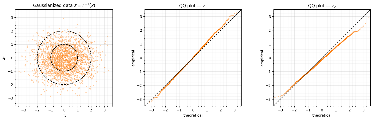
Clean: the latent fills the $\mathcal{N}(0,I)$ rings, the QQ plots sit on the diagonal, the skew is ~0 and there are no residual modes — the map that whitens a Gaussian is the affine family this flow spans, so the fit lands at the optimum (the log-det being exact helps the optimiser get there). Contrast the next section, where the target is not Gaussian.

4. The affine ceiling — two moons¶

Stacking matrix exponentials does not escape affine: a composition of linear maps is linear. So the moment the data is genuinely non-Gaussian, a MatrixExponential chain hits a wall. We fit the same chain to standardised two moons and look at the Gaussianized latent — it keeps the bimodal crescent structure that no affine map can remove.

Xm = make_moons(n_samples=2000, noise=0.06, random_state=0)[0]
Xm = jnp.asarray((Xm - Xm.mean(0)) / Xm.std(0))
moons_dist, _ = fit_chain(jr.key(1), Xm)
gxm, gym, densm = density_grid(moons_dist, lim=2.6)
Zm = gaussianize(moons_dist.bijection, Xm)

fig, (ax_d, ax_z) = plt.subplots(1, 2, figsize=(11.5, 5))
ax_d.contourf(np.asarray(gxm), np.asarray(gym), np.asarray(densm), levels=20, cmap="viridis")
ax_d.scatter(np.asarray(Xm[:, 0]), np.asarray(Xm[:, 1]), s=5, alpha=0.25, color="white", edgecolors="none")
ax_d.set(title="best affine fit to two moons\n(one Gaussian blob — misses both crescents)",
         xlabel="$x_1$", ylabel="$x_2$")
ax_d.set_aspect("equal"); style_ax(ax_d)
ax_z.scatter(Zm[:, 0], Zm[:, 1], color=LATENT_COLOR, **SCATTER_KW)
for r in (1.0, 2.0):
    ax_z.plot(r * np.cos(th), r * np.sin(th), **GAUSS_KW)
ax_z.set(title=r"Gaussianized latent $z=T^{-1}(x)$" + "\n(still two crescents — not $\\mathcal{N}(0,I)$)",
         xlabel="$z_1$", ylabel="$z_2$", xlim=(-3.6, 3.6), ylim=(-3.6, 3.6))
ax_z.set_aspect("equal"); style_ax(ax_z)
fig.tight_layout()
print(f"two-moons latent excess-kurtosis: z_1={stats.kurtosis(Zm[:, 0]):+.3f}, "
      f"z_2={stats.kurtosis(Zm[:, 1]):+.3f}  (non-zero => not Gaussianized)")

two-moons latent excess-kurtosis: z_1=-0.408, z_2=-1.273  (non-zero => not Gaussianized)

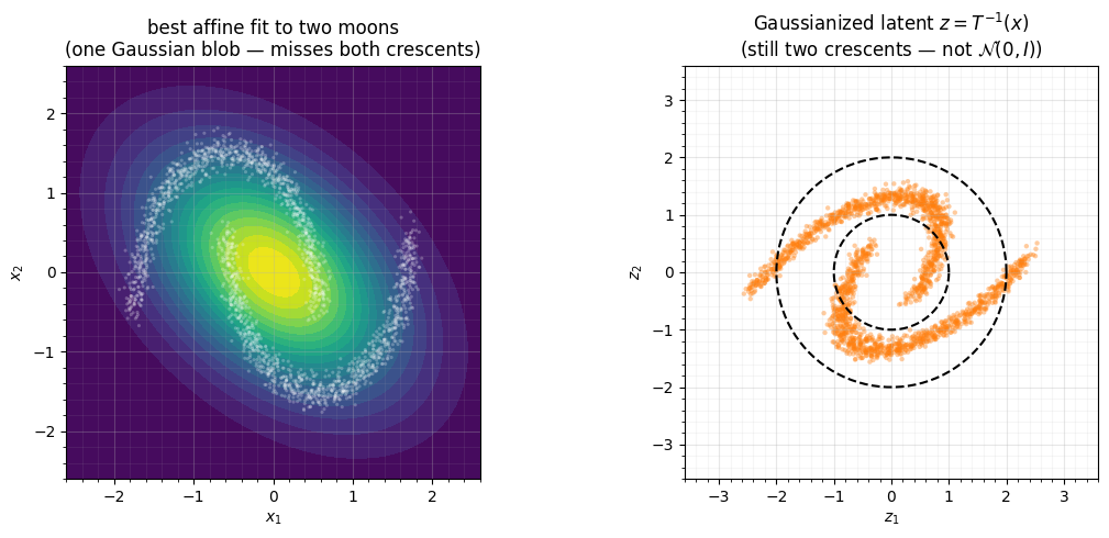
The density is a single tilted blob and the latent is still two crescents: an affine map cannot separate the modes. This is exactly why MatrixExponential earns its keep as a mixing block between nonlinear layers — the continuous-time analogue of a learned rotation in Part 2 — rather than as a stand-alone Gaussianizer. Slot a coupling or mixture-CDF layer (Parts 4-5) between two matrix-exponential blocks, or reach for FFJORD, and the modes come apart.

5. The $t$ -indexed family, for free¶

Because the bijection carries an explicit time, training at $t=1$ hands us the whole one-parameter family $p_t = (\exp(W_L t)\circ\cdots\circ\exp(W_1 t))_\#\, \mathcal{N}(0,I)$ — a smooth, exact interpolation from the base Gaussian at $t=0$ to the fitted target at $t=1$ , queryable at any $t$ with no retraining and no solver.

chain = gauss_dist.bijection
base = jr.normal(jr.key(17), (800, 2))
sweep = jnp.linspace(0.0, 1.0, 5)
fig, axes = plt.subplots(1, 5, figsize=(16, 3.6), sharex=True, sharey=True)
for ax, t in zip(axes, sweep):
    ct = pack_time_control(float(t))
    pushed = jax.vmap(lambda z: chain.transform_and_log_det(z, ct)[0])(base)
    ax.scatter(np.asarray(pushed[:, 0]), np.asarray(pushed[:, 1]), color=DATA_COLOR, **SCATTER_KW)
    ax.set(title=rf"$t={float(t):.2f}$", xlabel="$x_1$", xlim=(-3.5, 3.5), ylim=(-3.5, 3.5))
    ax.set_aspect("equal"); style_ax(ax)
axes[0].set_ylabel("$x_2$")
fig.suptitle(r"$p_t$: base $\mathcal{N}(0,I)$ at $t=0$ $\to$ anisotropic target at $t=1$ (exact, no ODE)", y=1.04)
fig.tight_layout()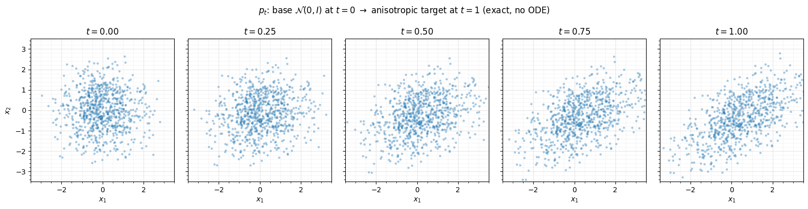

At $t=0$ the cloud is the base Gaussian; as $t\to1$ it tilts and stretches into the target — the matrix exponential delivers this interpolation in closed form.

Recap¶

	matrix-exponential flow	FFJORD (00–01)
flow map	$\exp(Wt)$ (closed form)	numerical ODE solve
log-det	exact $t\,\operatorname{tr}(W)$	trace integral, Hutchinson-estimated
per layer	affine in $x$	universal $f_\theta(t,x)$
Gaussianizes	a Gaussian, exactly	non-Gaussian data too
cost	dense matrix-exp, $O(d^3)$	many ODE steps × probes

The matrix-exponential flow is the linear corner of the continuous-time family: everything is closed-form and exact, the log-det is a one-liner, and it whitens a Gaussian perfectly — but it is affine, so it Gaussianizes only what a linear map can. Treat it as Part 2’s mixer made continuous, to be composed with the nonlinear blocks of Parts 4-5.

Next up. 03 — Latent ODE on spirals closes Part 6 by moving the dynamics into a latent space: encode, run an ODE on the latent state, decode — Gaussianization on the latent $z(0)$ — which is also the bridge to irregular time-series in Part 11.

References¶

Biloš, M., Sommer, J., Rangapuram, S. S., Januschowski, T., & Günnemann, S. (2021). Neural Flows: Efficient Alternative to Neural ODEs. Advances in Neural Information Processing Systems (NeurIPS).
Kidger, P. (2021). On Neural Differential Equations [Phdthesis]. University of Oxford.