FFJORD — continuous-time Gaussianization

00 — FFJORD: continuous-time Gaussianization¶

Every Gaussianization flow so far has been a finite stack: rotate, Gaussianize the margins, repeat $K$ times (Part 3), or stack $K$ coupling blocks and train end to end (Parts 4-5). Each block contributes an additive $\log|\det J|$ to the change-of-variables ledger. Now send the number of blocks to infinity and the per-block step to zero. The discrete composition $x_{k+1} = T_k(x_k)$ becomes an ordinary differential equation

\frac{\mathrm{d}x_t}{\mathrm{d}t} = f_\theta(t, x_t), \qquad t \in [0, 1],

((1))

and the stack of bijectors becomes the flow map of a single learned vector field $f_\theta$ — a continuous normalizing flow (CNF; Chen et al. 2018, FFJORD Grathwohl et al. (2019), Kidger (2021), Winkler et al. (2019)). The payoff is the instantaneous change of variables: where a discrete layer adds a log-determinant, the continuous flow integrates the trace of the Jacobian,

\frac{\mathrm{d}\log p_t(x_t)}{\mathrm{d}t} = -\operatorname{tr}\!\big(\partial_x f_\theta(t, x_t)\big) \;\;\Longrightarrow\;\; \log p_0(x_0) = \log p_1(x_1) + \int_0^1 \operatorname{tr}\!\big(\partial_x f_\theta(t, x_t)\big)\,\mathrm{d}t .

((2))

Two things follow. First, $f_\theta$ needs no architectural invertibility constraint — any smooth network will do, because the ODE flow is invertible by construction (run time backwards). Second, the log-det is a trace, not a determinant: cheap to evaluate exactly in low dimension and cheap to estimate in high dimension (notebook 01).

We follow the FlowJax convention where the base distribution is $\mathcal{N}(0,I)$ : the flow’s forward map (transform) integrates $t:0\to1$ and carries latent $\to$ data (generation), and its inverse integrates $t:1\to0$ and carries data $\to$ latent — the Gaussianization direction.

What you will see

A gf.FFJORD bijection with a small gf.DiffeqMLP vector field, trained by NLL.
The learned density and samples on two moons.
The Gaussianization check: push the data through the inverse flow and confirm the pushforward is $\mathcal{N}(0,I)$ (scatter, per-axis QQ, skew/kurtosis) — the Part 0 diagnostics, now on a continuous flow.
The transport: the vector field at three times, and data trajectories flowing onto the standard Gaussian.

import warnings

warnings.filterwarnings("ignore")

import diffrax
import equinox as eqx
import jax
import jax.numpy as jnp
import jax.random as jr
import matplotlib.pyplot as plt
import numpy as np
import optax
from flowjax.distributions import Normal, Transformed
from flowjax.train import fit_to_data
from scipy import stats
from sklearn.datasets import make_moons

import gauss_flows as gf
from _style import DATA_COLOR, GAUSS_KW, LATENT_COLOR, SCATTER_KW, style_ax

jax.config.update("jax_enable_x64", True)

1. Data¶

A standardised two-moons sample — the same toy used for the diagonal and coupling flows of Parts 4-5, so the comparison is honest. Standardisation matters here because the base distribution is a unit-variance Gaussian: without it the vector field would have to spend capacity undoing the scale.

n_samples = 1500
X_raw, _ = make_moons(n_samples=n_samples, noise=0.06, random_state=0)
X = (X_raw - X_raw.mean(0)) / X_raw.std(0)
X = jnp.asarray(X)

fig, ax = plt.subplots(figsize=(5.2, 5))
ax.scatter(np.asarray(X[:, 0]), np.asarray(X[:, 1]), color=DATA_COLOR, **SCATTER_KW)
ax.set(title="Two moons (standardised)", xlabel="$x_1$", ylabel="$x_2$")
ax.set_aspect("equal")
style_ax(ax)
fig.tight_layout()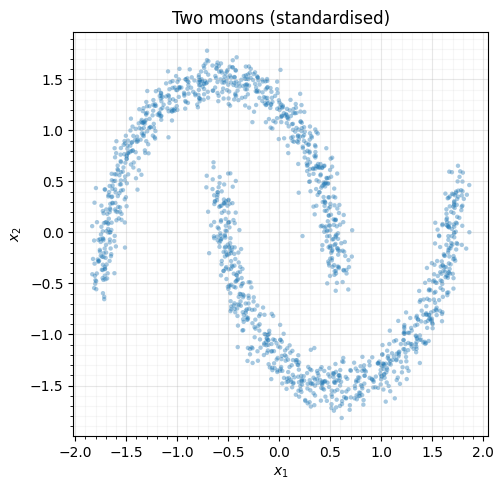

2. Build a FFJORD bijection¶

The vector field is a small gf.DiffeqMLP mapping $(t, x) \mapsto \dot x$ ; the gf.FFJORD bijection wraps it and hands the augmented dynamics $(\dot x, \dot{\log\det})$ to diffrax. The flow is unconditional (control_dim=0), so cond_shape is None and no condition is needed.

In 2-D the exact trace is essentially free — two Jacobian-vector products per ODE step — so we use divergence_mode="exact" for a variance-free log-det. (Notebook 01 is where the stochastic Hutchinson estimator earns its keep, as $d$ grows.)

key = jr.key(0)
vf_key, ffjord_key, train_key, sample_key = jr.split(key, 4)

vector_field = gf.DiffeqMLP(vf_key, in_dim=2, control_dim=0, hidden=(64, 64))

ffjord = gf.FFJORD(
    ffjord_key,
    shape=(2,),
    vector_field=vector_field,
    control_dim=0,
    divergence_mode="exact",
    solver="tsit5",
    adjoint="recursive_checkpoint",
    rtol=1e-4,
    atol=1e-4,
)
dist = Transformed(Normal(jnp.zeros(2)), ffjord)

n_params = sum(
    int(np.prod(p.shape))
    for p in jax.tree_util.tree_leaves(eqx.filter(vector_field, eqx.is_array))
)
print("unconditional FFJORD on shape (2,)")
print("  vector field        : DiffeqMLP, hidden=(64, 64)")
print(f"  trainable parameters: {n_params}")
print("  divergence mode     : exact (2 JVPs / ODE step in 2-D)")
print(f"  cond_shape          : {ffjord.cond_shape}")

unconditional FFJORD on shape (2,)
  vector field        : DiffeqMLP, hidden=(64, 64)
  trainable parameters: 4546
  divergence mode     : exact (2 JVPs / ODE step in 2-D)
  cond_shape          : None

3. Train by maximum likelihood¶

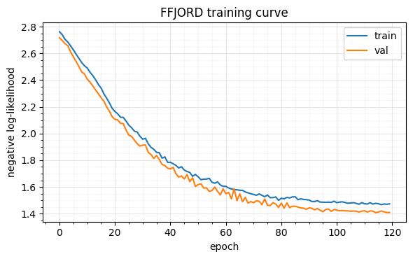
fit_to_data minimises the negative log-likelihood $-\frac1n\sum_i \log p_\theta(x_i)$ under the flow. Each gradient step solves a vmapped ODE over the batch, so FFJORD is far slower per step than the closed-form flows of Parts 4-5 — this is the slowest cell in the notebook. We cap it at ~120 epochs and use a cosine learning-rate decay ( $2\times10^{-3}\to{\sim}0$ ) so the fit settles inside that budget rather than crawling; early stopping on a validation split halts sooner if the held-out NLL plateaus, and gradient clipping guards against the occasional stiff ODE blowing up a gradient.

n_epochs, batch_size, val_prop = 120, 256, 0.1
steps_per_epoch = -(-int(X.shape[0] * (1 - val_prop)) // batch_size)  # ceil
lr = optax.cosine_decay_schedule(2e-3, decay_steps=n_epochs * steps_per_epoch, alpha=0.02)
optimizer = optax.chain(
    optax.clip_by_global_norm(5.0),
    optax.adam(lr),
)
trained_dist, losses = fit_to_data(
    train_key,
    dist,
    X,
    optimizer=optimizer,
    max_epochs=n_epochs,
    max_patience=20,
    batch_size=batch_size,
    val_prop=val_prop,
    show_progress=False,
)
print(f"stopped after {len(losses['train'])} epochs  "
      f"(best val NLL = {float(min(losses['val'])):.4f})")
trained_ffjord = trained_dist.bijection

fig, ax = plt.subplots(figsize=(6, 3.8))
ep = jnp.arange(len(losses["train"]))
ax.plot(ep, losses["train"], color=DATA_COLOR, label="train")
ax.plot(ep, losses["val"], color=LATENT_COLOR, label="val")
ax.set(xlabel="epoch", ylabel="negative log-likelihood", title="FFJORD training curve")
ax.legend()
style_ax(ax)
fig.tight_layout()

stopped after 120 epochs  (best val NLL = 1.4072)

4. Density and samples¶

For clean plots we re-instantiate the flow with the same trained vector field but a tighter solver and the direct adjoint (more accurate at eval time, when we don’t need backward gradients). The density on the left is $p_\theta$ on a grid; the right overlays fresh flow samples on the data.

exact_ffjord = gf.FFJORD(
    jr.key(99),  # trace_key unused in exact mode
    shape=(2,),
    vector_field=trained_ffjord.vector_field,
    control_dim=0,
    divergence_mode="exact",
    solver="tsit5",
    adjoint="direct",
    rtol=1e-6,
    atol=1e-6,
)
exact_dist = Transformed(Normal(jnp.zeros(2)), exact_ffjord)

lim, grid_n = 2.6, 70
xs = jnp.linspace(-lim, lim, grid_n)
gx, gy = jnp.meshgrid(xs, xs)
grid = jnp.stack([gx.ravel(), gy.ravel()], -1)


@eqx.filter_jit
def grid_log_prob(pts):
    return jax.vmap(exact_dist.log_prob)(pts)


density = jnp.exp(grid_log_prob(grid)).reshape(grid_n, grid_n)
samples = trained_dist.sample(sample_key, (n_samples,))

fig, (ax_d, ax_s) = plt.subplots(1, 2, figsize=(11.5, 5))
m = ax_d.contourf(np.asarray(gx), np.asarray(gy), np.asarray(density), levels=20, cmap="viridis")
ax_d.set(title=r"learned density $p_\theta(x)$", xlabel="$x_1$", ylabel="$x_2$")
ax_d.set_aspect("equal")
fig.colorbar(m, ax=ax_d, fraction=0.046)
style_ax(ax_d)

ax_s.scatter(np.asarray(X[:, 0]), np.asarray(X[:, 1]), color=DATA_COLOR, label="data", **SCATTER_KW)
ax_s.scatter(np.asarray(samples[:, 0]), np.asarray(samples[:, 1]), color="tab:red",
             marker="x", s=10, alpha=0.4, linewidths=0.7, label="flow samples")
ax_s.set(title="data vs. flow samples", xlabel="$x_1$", ylabel="$x_2$",
         xlim=(-lim, lim), ylim=(-lim, lim))
ax_s.set_aspect("equal")
ax_s.legend(loc="upper right", framealpha=0.9)
style_ax(ax_s)
fig.tight_layout()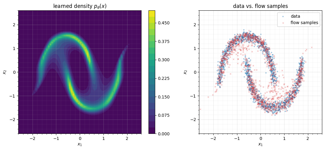

5. The Gaussianization check¶

Density and samples say the generative direction works. The Gaussianization direction is the inverse map $x \mapsto z$ (integrate $t:1\to0$ ): if the flow has learned the distribution, the pushforward of the data must be standard normal. We push the data through inverse_and_log_det and run the Part 0 diagnostics — a latent scatter against the $\mathcal{N}(0,I)$ contours, per-axis QQ plots, and the skew/kurtosis that should both sit at 0.

@eqx.filter_jit
def gaussianize(pts):
    return jax.vmap(lambda x: exact_ffjord.inverse_and_log_det(x)[0])(pts)


Z = np.asarray(gaussianize(X))

fig, axes = plt.subplots(1, 3, figsize=(15, 4.6))
# (a) latent scatter with N(0, I) reference rings
ax = axes[0]
ax.scatter(Z[:, 0], Z[:, 1], color=LATENT_COLOR, **SCATTER_KW)
th = np.linspace(0, 2 * np.pi, 200)
for r in (1.0, 2.0):
    ax.plot(r * np.cos(th), r * np.sin(th), **GAUSS_KW)
ax.set(title=r"Gaussianized data $z = T^{-1}(x)$", xlabel="$z_1$", ylabel="$z_2$",
       xlim=(-3.6, 3.6), ylim=(-3.6, 3.6))
ax.set_aspect("equal")
style_ax(ax)
# (b, c) per-axis QQ plots vs N(0, 1)
for j, ax in enumerate(axes[1:]):
    osm, osr = stats.probplot(Z[:, j], dist="norm", fit=False)
    ax.scatter(osm, osr, color=LATENT_COLOR, s=8, alpha=0.5, edgecolors="none")
    lo, hi = -3.5, 3.5
    ax.plot([lo, hi], [lo, hi], **GAUSS_KW)
    ax.set(title=f"QQ plot — $z_{j + 1}$", xlabel="theoretical", ylabel="empirical",
           xlim=(lo, hi), ylim=(lo, hi))
    ax.set_aspect("equal")
    style_ax(ax)
fig.tight_layout()

print("Gaussianized data moments (target: mean 0, std 1, skew 0, excess-kurt 0)")
for j in range(2):
    z = Z[:, j]
    print(f"  z_{j + 1}:  mean={z.mean():+.3f}  std={z.std():.3f}  "
          f"skew={stats.skew(z):+.3f}  exc-kurt={stats.kurtosis(z):+.3f}")

Gaussianized data moments (target: mean 0, std 1, skew 0, excess-kurt 0)
  z_1:  mean=-0.073  std=1.098  skew=-0.034  exc-kurt=-0.516
  z_2:  mean=+0.043  std=0.752  skew=+0.087  exc-kurt=+0.280

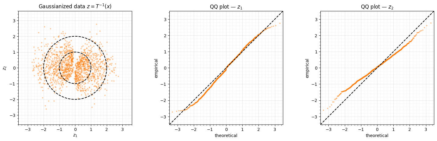
The latent points fill the $\mathcal{N}(0,I)$ rings, the QQ plots hug the diagonal, and the moments are close to $(0, 1, 0, 0)$ on both axes. The continuous flow has Gaussianized the two-moons data — the same target as RBIG and the coupling flows, reached by integrating an ODE rather than stacking blocks.

6. Watching the transport¶

What does the flow do? The vector field $f_\theta(t, x)$ is the velocity at each point and time; integrating it moves probability mass. We show it two ways. Left to right, the quivers are $f_\theta$ at $t = 0, \tfrac12, 1$ — the velocity field that the generation direction follows. Then we integrate the data backwards ( $t:1\to0$ ) with diffrax and watch the two crescents relax onto the standard Gaussian: the Gaussianization trajectory.

trained_vf = trained_ffjord.vector_field
qn = 19
qs = jnp.linspace(-lim, lim, qn)
qx, qy = jnp.meshgrid(qs, qs)
q_pts = jnp.stack([qx.ravel(), qy.ravel()], -1)

fig, axes = plt.subplots(1, 3, figsize=(15.5, 5.4), sharex=True, sharey=True)
for ax, t in zip(axes, (0.0, 0.5, 1.0)):
    vel = jax.vmap(lambda p: trained_vf(t, p, None))(q_pts)
    u = np.asarray(vel[:, 0]).reshape(qn, qn)
    v = np.asarray(vel[:, 1]).reshape(qn, qn)
    speed = np.hypot(u, v)
    ax.scatter(np.asarray(X[:, 0]), np.asarray(X[:, 1]), s=5, alpha=0.25,
               color="0.5", edgecolors="none", zorder=1)
    ax.quiver(np.asarray(qx), np.asarray(qy), u, v, speed, cmap="magma",
              width=0.004, zorder=2)
    ax.set(title=rf"$f_\theta(t={t},\, x)$", xlabel="$x_1$", xlim=(-lim, lim), ylim=(-lim, lim))
    ax.set_aspect("equal")
    style_ax(ax)
axes[0].set_ylabel("$x_2$")
fig.tight_layout()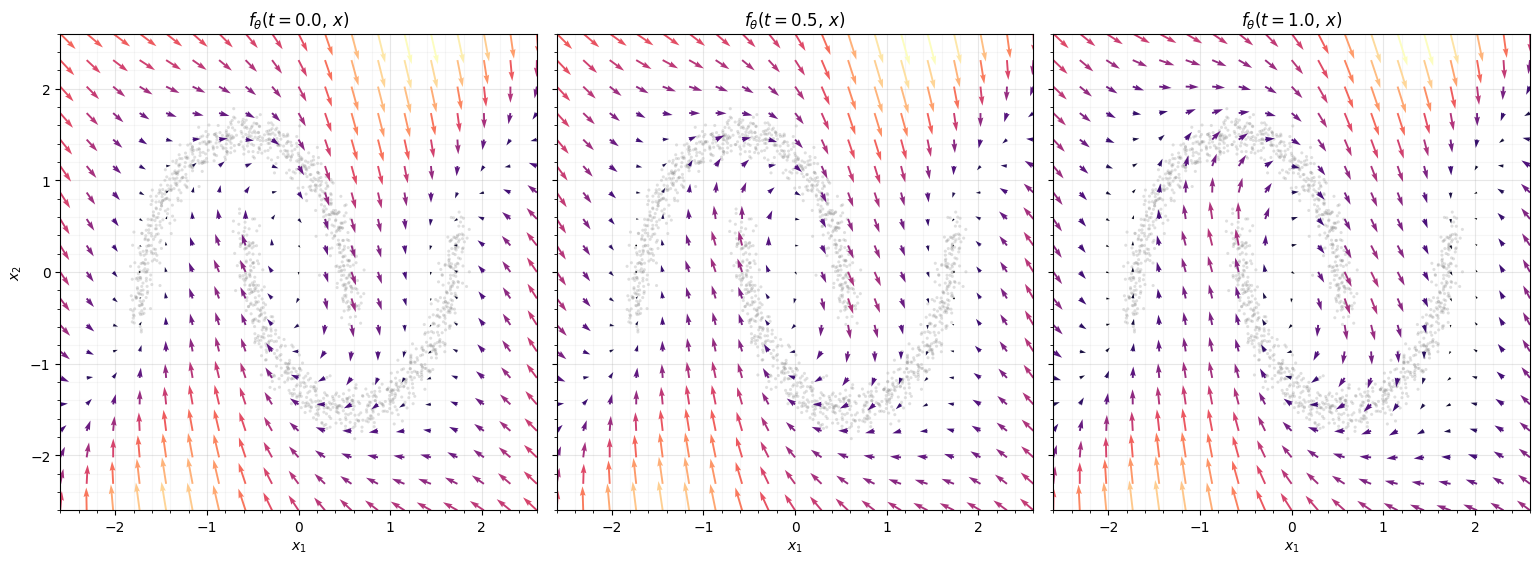

# Integrate the data backwards (t: 1 -> 0) along the trained vector field: the
# Gaussianization trajectory. We integrate the plain x-dynamics (no log-det
# augmentation needed for the path itself) directly with diffrax.
ts = jnp.linspace(1.0, 0.0, 6)
term = diffrax.ODETerm(lambda t, y, args: trained_vf(t, y, None))


@eqx.filter_jit
def trajectory(x0):
    sol = diffrax.diffeqsolve(
        term, diffrax.Tsit5(), t0=1.0, t1=0.0, dt0=-0.05, y0=x0,
        saveat=diffrax.SaveAt(ts=ts),
        stepsize_controller=diffrax.PIDController(rtol=1e-5, atol=1e-5),
    )
    return sol.ys


paths = np.asarray(jax.vmap(trajectory)(X[:600]))  # (600, len(ts), 2)

fig, axes = plt.subplots(1, len(ts), figsize=(18, 3.4), sharex=True, sharey=True)
for k, ax in enumerate(axes):
    ax.scatter(paths[:, k, 0], paths[:, k, 1], color=LATENT_COLOR, s=7, alpha=0.4,
               edgecolors="none")
    for r in (1.0, 2.0):
        ax.plot(r * np.cos(th), r * np.sin(th), color="0.3", lw=1.0, ls="--", alpha=0.6)
    ax.set(title=f"$t = {float(ts[k]):.1f}$", xlim=(-3.4, 3.4), ylim=(-3.4, 3.4))
    ax.set_aspect("equal")
    ax.set_xticks([]); ax.set_yticks([])
axes[0].set_ylabel("data → $\\mathcal{N}(0,I)$")
fig.suptitle("Gaussianization trajectory: integrating the data backwards along $f_\\theta$", y=1.04)
fig.tight_layout()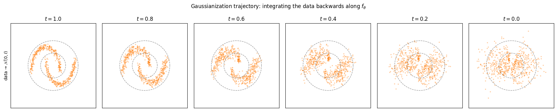

At $t=1$ the points are the two crescents; as $t\to0$ the vector field straightens and spreads them into an isotropic Gaussian blob inside the reference rings. This is the continuous analogue of the per-layer pushforward in Part 4’s layer-wise inspection — a smooth path instead of discrete jumps.

7. The cost of the log-det — a forward pointer¶

Everything above used the exact trace, which is fine in 2-D. The exact trace costs $d$ Jacobian-vector products per ODE step, so it scales as $O(d)$ per step — tolerable here, prohibitive for images. The next notebook replaces it with Hutchinson’s estimator, $\operatorname{tr}(A)\approx z^\top A z$ for a random probe $z$ , an $O(1)$ -per-step stochastic trace that is what lets free-form CNFs scale. A quick taste of the trade-off on the trained flow:

eval_pts = X[:300]
exact_lp = jax.vmap(exact_dist.log_prob)(eval_pts)


def hutch_log_prob(n_probes, seed):
    bij = gf.FFJORD(
        jr.key(seed), shape=(2,), vector_field=trained_ffjord.vector_field,
        control_dim=0, divergence_mode="hutchinson", n_hutchinson_samples=n_probes,
        solver="tsit5", adjoint="direct", rtol=1e-5, atol=1e-5,
    )
    return jax.vmap(Transformed(Normal(jnp.zeros(2)), bij).log_prob)(eval_pts)


print(f"exact   mean log p = {float(jnp.mean(exact_lp)):+.4f}  (reference)\n")
print(f"{'n_probes':>9s}  {'mean log p':>11s}  {'bias':>9s}  {'RMSE':>8s}")
for n in (1, 4, 16, 64):
    lp = hutch_log_prob(n, 1234 + n)
    bias = float(jnp.mean(lp - exact_lp))
    rmse = float(jnp.sqrt(jnp.mean((lp - exact_lp) ** 2)))
    print(f"{n:>9d}  {float(jnp.mean(lp)):>+11.4f}  {bias:>+9.4f}  {rmse:>8.4f}")

exact   mean log p = -1.5672  (reference)

 n_probes   mean log p       bias      RMSE

        1      -0.9277    +0.6395    2.5668

        4      -1.8870    -0.3197    1.2834

       16      -1.9669    -0.3997    1.6043

       64      -1.5472    +0.0200    0.0802

Even a single probe gives a sensible mean NLL (the per-point variance cancels in the average), but the per-point RMSE shrinks like $1/\sqrt{n}$ — which matters for anomaly scoring. Notebook 01 makes this precise.

Recap¶

	discrete stack (Parts 4-5)	continuous flow (FFJORD)
map	$x_{k+1} = T_k(x_k)$ , $K$ blocks	$\dot x = f_\theta(t, x)$ , one vector field
log-det	$\sum_k \log\lvert\det J_{T_k}\rvert$	$-\int_0^1 \operatorname{tr}(\partial_x f_\theta)\,\mathrm{d}t$
invertibility	architectural (triangular / orthogonal)	free — run the ODE backwards
cost	closed-form per block	ODE solve per evaluation; trace per step

A FFJORD is the infinite-depth limit of a Gaussianization stack: drop the architectural invertibility constraint, pay for it with an ODE solve, and earn an arbitrarily flexible vector field whose log-det is a trace. We confirmed it Gaussianizes two moons onto $\mathcal{N}(0,I)$ — the same target, a different machine.

Next up. The trace is the whole game. 01 — Hutchinson trace estimator shows how to estimate it in $O(1)$ instead of $O(d)$ , the bias/variance of the estimate, and when the exact trace is still worth it.

References¶

Grathwohl, W., Chen, R. T. Q., Bettencourt, J., Sutskever, I., & Duvenaud, D. (2019). FFJORD: Free-Form Continuous Dynamics for Scalable Reversible Generative Models. International Conference on Learning Representations (ICLR).
Kidger, P. (2021). On Neural Differential Equations [Phdthesis]. University of Oxford.
Winkler, C., Worrall, D. E., Hoogeboom, E., & Welling, M. (2019). Learning Likelihoods with Conditional Normalizing Flows. arXiv Preprint arXiv:1912.00042.