Composition & the additive log-determinant

01 — Composition & the additive log-determinant¶

Notebook 00 gave us one invertible map and its $\log|\det J|$ . But a single elementwise CDF or a single rotation cannot turn a tangled 2D distribution into a standard Gaussian — we need to stack many simple maps into a deep one. The reason stacking is cheap, and the reason normalizing flows exist at all Rezende & Mohamed (2015)Dinh et al. (2017), is a one-line consequence of the chain rule: when you compose maps, their log-determinants add.

What you will see

The composition rule $\log|\det J_T| = \sum_k \log|\det J_{T_k}(x_{k-1})|$ derived from $\det(AB) = \det A \det B$ .
A from-scratch check: the running-intermediate sum equals the autodiff log-det of the whole composition.
Why the intermediates matter — evaluating every term at the input $x_0$ gives the wrong answer for nonlinear maps.
A stack of gauss_flows (rotation, marginal) blocks accumulating its log-det layer by layer, with the orthogonal rotations contributing 0.

import warnings

warnings.filterwarnings("ignore")

import jax
import jax.numpy as jnp
import jax.random as jr
import matplotlib.pyplot as plt
import numpy as np

from _style import style_ax

jax.config.update("jax_enable_x64", True)
rng = np.random.default_rng(1)

1. The composition rule¶

Write a deep map as a composition of $K$ bijectors,

T = T_K \circ T_{K-1} \circ \cdots \circ T_1, \qquad x_0 = x,\quad x_k = T_k(x_{k-1}),\quad z = x_K.

((1))

By the chain rule the Jacobian of the whole map is a product of the per-layer Jacobians, each evaluated at the intermediate point it acts on:

J_T(x) = J_{T_K}(x_{K-1})\, J_{T_{K-1}}(x_{K-2}) \cdots J_{T_1}(x_0).

((2))

Determinants turn products into products, $\det(AB)=\det A \det B$ , and logs turn products into sums:

\boxed{\;\log\big|\det J_T(x)\big| = \sum_{k=1}^{K} \log\big|\det J_{T_k}(x_{k-1})\big|\;}

((3))

So the cost of a deep flow’s log-det is just the sum of cheap per-layer log-dets — no giant $d\times d$ determinant of the composition is ever formed. The one subtlety the boxed formula encodes: the $k$ -th term is evaluated at $x_{k-1}$ , the running state entering layer $k$ , not at the original input.

2. Verify it from scratch¶

Take three simple invertible maps — an affine mixer, an elementwise nonlinearity, and another affine — and compose them. We compare two ways of getting the total log-det:

Whole-composition autodiff: build $T$ , differentiate it, slogdet.
Running-intermediate sum: walk the layers, summing each layer’s log-det evaluated at the state entering it.

A1 = jnp.asarray(rng.standard_normal((2, 2)) * 0.5 + jnp.eye(2))
A2 = jnp.asarray(rng.standard_normal((2, 2)) * 0.5 + jnp.eye(2))
b1 = jnp.asarray(rng.standard_normal(2))


def layer1(x):
    return A1 @ x + b1


def layer2(x):
    return jnp.tanh(0.8 * x) + 0.3 * x  # elementwise, monotone => invertible


def layer3(x):
    return A2 @ x


layers = [layer1, layer2, layer3]


def compose(fns):
    def T(x):
        for f in fns:
            x = f(x)
        return x
    return T


def layer_logdet(f, x):
    return jnp.linalg.slogdet(jax.jacfwd(f)(x))[1]


x = jnp.asarray(rng.standard_normal(2))

# (1) whole-composition autodiff
logdet_full = jnp.linalg.slogdet(jax.jacfwd(compose(layers))(x))[1]

# (2) running-intermediate sum
total, xk = 0.0, x
for f in layers:
    total = total + layer_logdet(f, xk)
    xk = f(xk)

print(f"whole-composition autodiff log|det J| = {logdet_full:.8f}")
print(f"running-intermediate sum             = {total:.8f}")
print(f"absolute difference                  = {abs(logdet_full - total):.2e}")
assert jnp.allclose(logdet_full, total, atol=1e-8)
print("\n[ok] composition => log-determinants add.")

whole-composition autodiff log|det J| = -0.50001264
running-intermediate sum             = -0.50001264
absolute difference                  = 2.22e-16

[ok] composition => log-determinants add.

3. The intermediates matter¶

The boxed formula evaluates layer $k$ ’s log-det at the running state $x_{k-1}$ . A common slip is to evaluate every layer at the original input $x_0$ . For the linear layers that happens to be fine (their Jacobian is constant), but the nonlinear layer2 has a Jacobian that depends on where it is evaluated — so the shortcut is wrong.

wrong = sum(layer_logdet(f, x) for f in layers)  # all evaluated at x0 (WRONG)
print(f"correct (running intermediates) = {total:.8f}")
print(f"wrong   (all at x0)             = {wrong:.8f}")
print(f"discrepancy from nonlinearity  = {abs(total - wrong):.4f}")

correct (running intermediates) = -0.50001264
wrong   (all at x0)             = -0.35780308
discrepancy from nonlinearity  = 0.1422

The gap is entirely due to layer2: feeding it $x_0$ instead of $x_1 = \text{layer1}(x_0)$ evaluates its stretch factor at the wrong point. Flow libraries get this right by construction — each bijector receives the output of the previous one.

4. The log-density of a deep flow¶

Combining with the change-of-variables identity from notebook 00, a deep flow that maps data $x$ to latent $z = T(x)$ with base $p_Z = \mathcal{N}(0, I)$ scores a point as

\log p_X(x) = \log p_Z\big(T(x)\big) + \sum_{k=1}^{K}\log\big|\det J_{T_k}(x_{k-1})\big|.

((4))

Every layer contributes one additive term. Layers with $\log|\det J| = 0$ — orthogonal rotations are the canonical example — change the geometry for free, contributing nothing to the density bookkeeping. That is exactly why Gaussianization alternates rotations (free, redistribute mass across axes) with marginal transforms (do the density work). We see this next.

5. The bridge: a stack of `gauss_flows` blocks¶

A Gaussianization flow is a Chain of (rotation, marginal) blocks. Each gauss_flows bijector exposes transform_and_log_det, and flowjax.bijections.Chain composes them with exactly the additive rule from §1. We build the stack by hand, push a batch of 2D data through it, and record each sub-layer’s mean log-det contribution.

import gauss_flows as gf
from flowjax.bijections import Chain

# A correlated, skewed 2D dataset (banana-ish) to push through the stack.
key = jr.key(0)
u = rng.standard_normal((4000, 2))
data = np.stack([u[:, 0], u[:, 1] + 0.4 * u[:, 0] ** 2 - 0.4], axis=1)
data = jnp.asarray((data - data.mean(0)) / data.std(0))

n_blocks = 4
bijectors, labels = [], []
for k in range(n_blocks):
    bijectors += [gf.HouseholderRotation(n_reflections=2, shape=(2,)),
                  gf.MixtureGaussianCDF(n_components=8, shape=(2,))]
    labels += [f"rot {k}", f"marg {k}"]

chain = Chain(bijectors)

# Per-sub-layer mean log-det, walking the running intermediates over the batch.
per_layer = []
xk = data
for bij in bijectors:
    yk, ldj = jax.vmap(bij.transform_and_log_det)(xk)
    per_layer.append(float(jnp.mean(ldj)))
    xk = yk

# Cross-check: the hand-walked sum equals Chain's own log-det (mean over batch).
_, ldj_chain = jax.vmap(chain.transform_and_log_det)(data)
print(f"sum of per-layer mean log-dets = {np.sum(per_layer):.6f}")
print(f"Chain mean log-det             = {float(jnp.mean(ldj_chain)):.6f}")
assert jnp.allclose(np.sum(per_layer), float(jnp.mean(ldj_chain)), atol=1e-6)
print("[ok] Chain accumulates the additive log-det we derived by hand.")

sum of per-layer mean log-dets = -2.406725
Chain mean log-det             = -2.406725
[ok] Chain accumulates the additive log-det we derived by hand.

fig, ax = plt.subplots(figsize=(9, 4))
colors = ["tab:gray" if "rot" in l else "tab:orange" for l in labels]
ax.bar(range(len(per_layer)), per_layer, color=colors)
ax.axhline(0, color="k", lw=0.8)
ax.plot(range(len(per_layer)), np.cumsum(per_layer), "-o", color="tab:blue",
        lw=1.5, ms=4, label="cumulative log-det")
ax.set_xticks(range(len(labels)))
ax.set_xticklabels(labels, rotation=45, ha="right")
ax.set(ylabel=r"mean $\log|\det J|$ contribution",
       title="Per-layer log-det: rotations are free, marginals do the work")
ax.legend()
style_ax(ax)
fig.tight_layout()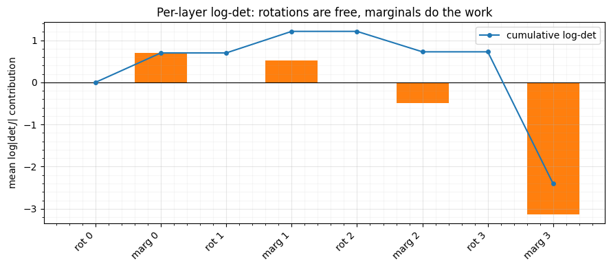

The grey rotation bars sit at exactly 0 — orthogonal maps have $|\det J| = 1$ , so they cost nothing in the density ledger. The orange marginal bars carry the entire log-det, and the blue line is their running total: precisely the $\sum_k \log|\det J_{T_k}|$ a single chain.log_prob call would add to $\log p_Z(z)$ .

This decomposition is not just diagnostic. It is how every flow in this curriculum computes a density — and it is why gf.gaussianization_flow(...), which wraps this very Chain, satisfies flow.log_prob(x) == flow.base_dist.log_prob(z) + log_det with z, log_det = flow.bijection.inverse_and_log_det(x).

Recap¶

concept	formula	in code
composition Jacobian	$J_T = J_{T_K}\cdots J_{T_1}$ (chain rule)	`jax.jacfwd(compose(layers))`
additive log-det	$\log\lvert\det J_T\rvert=\sum_k\log\lvert\det J_{T_k}(x_{k-1})\rvert$	running sum over layers
deep-flow log-density	$\log p_Z(z)+\sum_k\log\lvert\det J_{T_k}\rvert$	`flow.log_prob(x)`
rotations are free	orthogonal $\Rightarrow\log\lvert\det J\rvert=0$	grey bars at 0
the library does it	additive rule inside `Chain`/`Scan`	`Chain(bijectors)`

Next up. We have built maps in the data→latent direction. But which direction should a flow store and which should it compute? In 02 — Forward vs. inverse parameterisation we see how that single choice splits flows into “good at density estimation” vs. “good at fast sampling”.

References¶

Rezende, D. J., & Mohamed, S. (2015). Variational Inference with Normalizing Flows. International Conference on Machine Learning (ICML).
Dinh, L., Sohl-Dickstein, J., & Bengio, S. (2017). Density Estimation using Real NVP. International Conference on Learning Representations (ICLR).

Composition & the additive log-determinant

01 — Composition & the additive log-determinant¶

1. The composition rule¶

2. Verify it from scratch¶

3. The intermediates matter¶

4. The log-density of a deep flow¶

5. The bridge: a stack of gauss_flows blocks¶

Recap¶

5. The bridge: a stack of `gauss_flows` blocks¶