Gaussianity diagnostics - Research Notebook

06 — Gaussianity diagnostics¶

We can build a density destructor (notebook 04) and trust its arithmetic (notebook 05). The last foundational question is how do we know it worked? — that the pushforward $z = T(x)$ really is $\mathcal{N}(0, I)$ . Gaussianity has two levels, and we need a diagnostic for each: per-coordinate (are the marginals standard normal?) and joint (is the whole vector multivariate normal, i.e. also independent across coordinates?).

What you will see

Marginal: QQ-plots and skewness / excess-kurtosis, before vs. after.
Negentropy as the information-theoretic non-Gaussianity — RBIG’s classic stopping signal — and why it is noisy to estimate near convergence.
Joint: an energy-distance test against $\mathcal{N}(0, I)$ that falls monotonically as RBIG adds layers (Henze–Zirkler is the classical alternative).

import warnings

warnings.filterwarnings("ignore")

import matplotlib.pyplot as plt
import numpy as np
from scipy import stats
from sklearn.datasets import make_moons

import rbig
from _style import GAUSS_KW, style_ax

rng = np.random.default_rng(7)

X, _ = make_moons(5000, noise=0.06, random_state=0)
X = (X - X.mean(0)) / X.std(0)

# Fit a density destructor and grab the pushforward + intermediate states.
model = rbig.AnnealedRBIG(n_layers=50, rotation="random", random_state=0)
model.fit(X)


def through_layers(k):
    s = X
    for layer in model.layers_[:k]:
        s = layer.transform(s)
    return s


Z = through_layers(len(model.layers_))  # fully Gaussianized

1. Marginal diagnostics: QQ-plots and moments¶

The first, cheapest check is per-coordinate. A QQ-plot sorts the samples and plots them against the matching standard-normal quantiles $\Phi^{-1}((i - 0.5)/n)$ ; if the coordinate is $\mathcal{N}(0,1)$ the points fall on the identity line. Two scalar summaries back it up: skewness $\gamma_1$ (asymmetry) and excess kurtosis $\gamma_2$ (tail weight), both 0 for a Gaussian.

def qq(ax, samples, title):
    s = np.sort(samples)
    q_theory = stats.norm.ppf((np.arange(1, len(s) + 1) - 0.5) / len(s))
    ax.plot([-4, 4], [-4, 4], **GAUSS_KW, label="$y=x$ (Gaussian)")
    ax.plot(q_theory, s, ".", ms=2, alpha=0.4, color="tab:blue")
    ax.set(title=title, xlabel="theoretical $\\Phi^{-1}$ quantile",
           ylabel="sample quantile", xlim=(-4, 4), ylim=(-4, 4))
    ax.set_aspect("equal")
    ax.legend(loc="upper left", fontsize=8)
    style_ax(ax)


fig, axes = plt.subplots(1, 2, figsize=(10, 4.6))
qq(axes[0], X[:, 0], "data: coordinate $x_1$")
qq(axes[1], Z[:, 0], r"Gaussianized: $z_1$")
fig.tight_layout()

print(f"{'':12s}{'skewness':>12s}{'excess kurtosis':>18s}")
for name, d in [("data x", X), ("Gaussianized z", Z)]:
    print(f"{name:12s}{np.abs(stats.skew(d)).mean():12.4f}"
          f"{np.abs(stats.kurtosis(d)).mean():18.4f}")

                skewness   excess kurtosis
data x            0.0006            1.0627
Gaussianized z      0.0003            0.0109

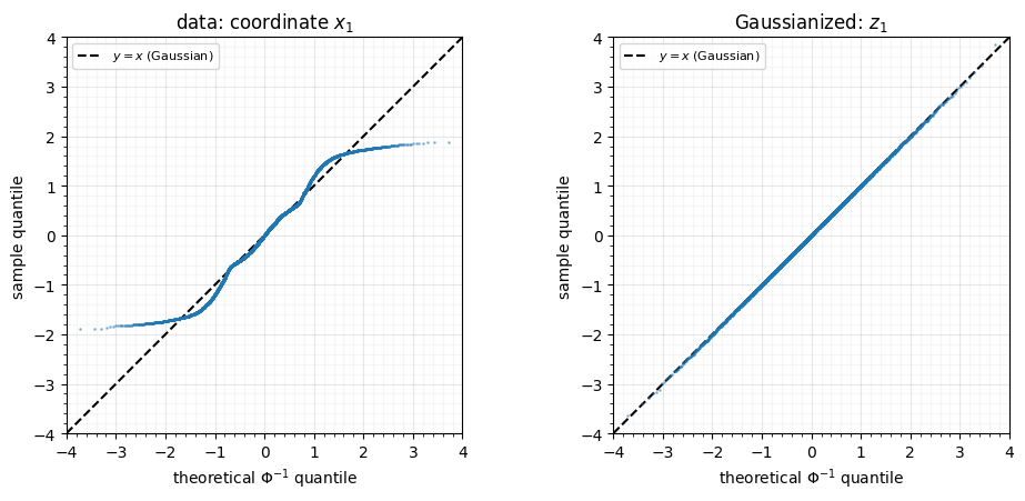
The data QQ-plot is S-shaped — the two-moons marginal is platykurtic (light tails, excess kurtosis $< 0$ ) and bends away from the line. After Gaussianization the points snap onto $y = x$ , and the mean $|\gamma_1|, |\gamma_2|$ both collapse toward 0. QQ-plots catch what kind of non-Gaussianity remains (skew vs. tails); the moments put a number on it.

2. Negentropy: the information-theoretic stopping signal¶

Moments only probe the 3rd and 4th order. The complete per-coordinate non-Gaussianity is the negentropy $J(p) = H(\mathcal{N}_{\sigma}) - H(p) \ge 0$ from notebook 03, and the complete joint non-Gaussianity is the KL to the standard normal, which decomposes as

\mathrm{KL}\big(p \,\|\, \mathcal{N}(0, I)\big) = \underbrace{\mathrm{TC}(p)}_{\text{dependence}} + \underbrace{\textstyle\sum_i J(p_i)}_{\text{marginal non-Gaussianity}}.

((1))

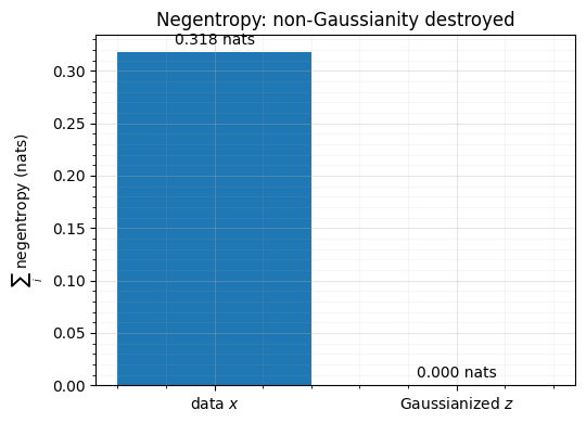
Driving this to 0 is the RBIG objective, and rbig uses the per-layer information reduction as its stopping criterion Laparra et al. (2011). We estimate negentropy with rbig.negentropy on the data and on the pushforward.

neg_data = float(np.sum(np.clip(rbig.negentropy(X), 0, None)))
neg_gauss = float(np.sum(np.clip(rbig.negentropy(Z), 0, None)))
print(f"sum negentropy  — data        : {neg_data:.4f} nats")
print(f"sum negentropy  — Gaussianized: {neg_gauss:.4f} nats  (~0)")

fig, ax = plt.subplots(figsize=(5.5, 4))
bars = ax.bar(["data $x$", "Gaussianized $z$"], [neg_data, neg_gauss],
              color=["tab:blue", "tab:green"])
ax.bar_label(bars, fmt="%.3f nats", padding=3)
ax.set(ylabel=r"$\sum_i$ negentropy (nats)",
       title="Negentropy: non-Gaussianity destroyed")
style_ax(ax)
fig.tight_layout()

sum negentropy  — data        : 0.3181 nats
sum negentropy  — Gaussianized: 0.0001 nats  (~0)

3. Joint normality: an energy-distance test¶

Marginal checks can all pass while the joint is still structured (think of a rotated non-Gaussian whose axes happen to look normal). For the joint verdict we compare the pushforward $Z$ to a fresh $\mathcal{N}(0, I)$ sample with the energy distance — a kernel two-sample statistic that is 0 iff the two distributions match:

\mathcal{E}(Z, G) = 2\,\mathbb{E}\lVert Z - G\rVert - \mathbb{E}\lVert Z - Z'\rVert - \mathbb{E}\lVert G - G'\rVert \;\ge\; 0.

((2))

(The classical Henze–Zirkler test is the textbook alternative Cover & Thomas (2006); the energy distance is easy to compute from scratch and needs no distributional table.) We track it as RBIG adds layers.

def energy_distance(A, B):
    """Multivariate energy distance between samples A and B (>= 0, 0 iff equal)."""
    def mean_pairwise(P, Q):
        return np.sqrt(((P[:, None, :] - Q[None, :, :]) ** 2).sum(-1)).mean()
    return (2 * mean_pairwise(A, B)
            - mean_pairwise(A, A) - mean_pairwise(B, B))


def avg_energy(state, n_draws=6, n=800):
    """Average the energy distance over several N(0,I) draws to tame estimator noise."""
    vals = []
    for _ in range(n_draws):
        idx = rng.choice(len(state), n, replace=False)
        vals.append(max(energy_distance(state[idx], rng.standard_normal((n, 2))), 0.0))
    return float(np.mean(vals))


layers = np.arange(0, len(model.layers_) + 1, 2)
energy = np.array([avg_energy(through_layers(k)) for k in layers])

print(f"energy distance to N(0,I):  data = {energy[0]:.4f}  ->  "
      f"final = {energy[-1]:.4f}  (sampling floor)")

fig, ax = plt.subplots(figsize=(7.5, 4.2))
ax.plot(layers, energy, "-o", color="tab:purple", ms=4)
ax.axhline(energy[-5:].mean(), color="k", ls="--", lw=1,
           label="sampling floor (two N(0,I) samples)")
ax.set(xlabel="RBIG layers applied", ylabel=r"energy distance to $\mathcal{N}(0,I)$",
       title="Joint Gaussianity improves with depth, then hits the floor")
ax.legend()
style_ax(ax)
fig.tight_layout()

energy distance to N(0,I):  data = 0.0497  ->  final = 0.0030  (sampling floor)

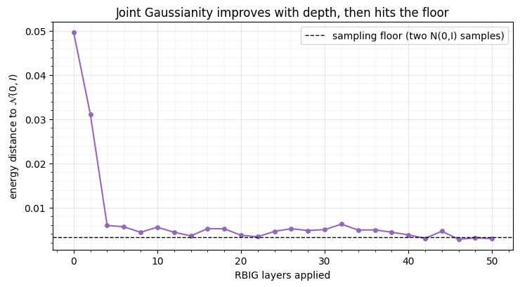
The energy distance falls steadily from the tangled two-moons toward the noise floor (the residual is the finite-sample distance between two genuine $\mathcal{N}(0, I)$ samples). This is the joint analogue of the per-layer information reduction: a single, robust number that says “keep adding layers” until it stops dropping — the practical stopping rule when negentropy is too noisy to trust.

Recap¶

level	diagnostic	Gaussian value	tool
marginal shape	QQ-plot	points on $y=x$	`numpy` + `scipy.stats`
marginal moments	skewness, excess kurtosis	$0,\ 0$	`scipy.stats.skew/kurtosis`
marginal info	negentropy $J(p_i)$	0	`rbig.negentropy`
dependence	total correlation	0	`rbig.total_correlation`
joint	energy distance / Henze–Zirkler	0	from scratch

References¶

Laparra, V., Camps-Valls, G., & Malo, J. (2011). Iterative Gaussianization: From ICA to Random Rotations. IEEE Transactions on Neural Networks, 22(4), 537–549. 10.1109/TNN.2011.2106511
Cover, T. M., & Thomas, J. A. (2006). Elements of Information Theory (2nd ed.). Wiley-Interscience.