RBIG warm-start for coupling flows

05 — RBIG warm-start for coupling flows¶

Part 4, notebook 01 warm-started a diagonal flow from a greedy RBIG fit. Coupling flows (notebook 04) are more expressive, but that expressiveness makes them harder to train from a random start: the conditioner MLP begins random, so each coupling transform is a random function of the other coordinates — the optimiser first has to discover that the conditioner should be doing anything sensible at all.

gauss_flows.fit_rbig_coupling warm-starts a coupling flow too, and it does so with a beautiful trick — the zero-kernel contract (the data-dependent / zero-init idea of Glow Kingma & Dhariwal (2018)). Right after the greedy fit, every coupling’s conditioner has a zero final-layer kernel, so it ignores its input and emits only its bias. A coupling whose conditioner outputs a constant is exactly a diagonal marginal (the RBIG fit of notebook 01) on its active half. So the warm-started coupling flow starts life as a diagonal RBIG flow, and gradient training switches on the conditioner from there — the coupling↔diagonal equivalence made concrete.

What you will see

fit_rbig_coupling warm-start vs a matched random-init coupling flow.
The zero-kernel contract verified: conditioner kernels are exactly 0 at init, non-zero after training.
Cold vs warm training at an equal budget — the warm start is ahead the whole way and lands at a better optimum.

import warnings

warnings.filterwarnings("ignore")

import equinox as eqx
import jax
import jax.numpy as jnp
import jax.random as jr
import matplotlib.pyplot as plt
import numpy as np
import optax
from flowjax.bijections import Chain, Flip, Invert
from flowjax.distributions import Normal, Transformed
from sklearn.datasets import make_moons

import gauss_flows as gf
from gauss_flows import MixtureGaussianCDFCoupling
from gauss_flows._src.transforms.bijections.coupling.mixture_cdf import (
    MixtureGaussianCDFCoupling as _CouplingClass,
)
from gauss_flows._src.transforms.bijections.linear.rotation import HouseholderRotation
from _style import SCATTER_KW, style_ax

jax.config.update("jax_enable_x64", True)

X, _ = make_moons(n_samples=3000, noise=0.06, random_state=0)
X = jnp.asarray((X - X.mean(0)) / X.std(0))

N_BLOCKS, N_COMPONENTS, NN_WIDTH, NN_DEPTH = 4, 8, 64, 2


def train_flow(flow, *, steps, peak_lr, clip_norm=1.0, batch=512, seed=1):
    """NLL training: optax with gradient clipping + one-cycle cosine LR."""
    params, static = eqx.partition(flow, eqx.is_inexact_array)
    schedule = optax.cosine_onecycle_schedule(transition_steps=steps, peak_value=peak_lr)
    opt = optax.chain(optax.clip_by_global_norm(clip_norm), optax.adam(schedule))
    state = opt.init(params)

    @eqx.filter_jit
    def step(params, state, xb):
        loss, grads = eqx.filter_value_and_grad(
            lambda p: -jnp.mean(jax.vmap(eqx.combine(p, static).log_prob)(xb)))(params)
        updates, state = opt.update(grads, state)
        return eqx.apply_updates(params, updates), state, loss

    key, traj = jr.key(seed), []
    for i in range(steps):
        key, sk = jr.split(key)
        idx = jr.randint(sk, (batch,), 0, X.shape[0])
        params, state, loss = step(params, state, X[idx])
        if i % 25 == 0:
            traj.append(float(loss))
    return eqx.combine(params, static), np.array(traj)


logp = lambda flow: float(jax.vmap(flow.log_prob)(X).mean())

1. Warm-start vs random-init coupling¶

fit_rbig_coupling greedily fits a mixture-CDF coupling flow. For a fair comparison we build a random-init flow with the same architecture (the public coupling_gaussianization_flow uses spline couplings, so we assemble the matching mixture-CDF stack directly). Both are Invert-wrapped Chains of rotation + coupling blocks.

def random_coupling_flow(key, n_blocks, n_components):
    """A random-init mixture-CDF coupling flow matching fit_rbig_coupling's stack."""
    bijections = []
    for k in jr.split(key, n_blocks):
        rk, ck1, ck2 = jr.split(k, 3)
        rot = HouseholderRotation(n_reflections=2, shape=(2,))
        rot = eqx.tree_at(lambda r: r.params, rot, jr.normal(rk, rot.params.shape))
        coupling_kw = dict(shape=(2,), n_components=n_components,
                           nn_width=NN_WIDTH, nn_depth=NN_DEPTH)
        bijections += [rot,
                       MixtureGaussianCDFCoupling(ck1, **coupling_kw),
                       Flip(shape=(2,)),
                       MixtureGaussianCDFCoupling(ck2, **coupling_kw),
                       Flip(shape=(2,))]
    return Transformed(Normal(jnp.zeros(2)), Invert(Chain(bijections)))


cold_init = random_coupling_flow(jr.key(3), N_BLOCKS, N_COMPONENTS)
warm_init = gf.fit_rbig_coupling(X, jr.key(3), n_layers=N_BLOCKS, n_components=N_COMPONENTS,
                                 nn_width=NN_WIDTH, nn_depth=NN_DEPTH)

print(f"coupling log p at init:  random = {logp(cold_init):+.3f}   "
      f"RBIG warm = {logp(warm_init):+.3f}  (improvement {logp(warm_init) - logp(cold_init):+.3f})")

coupling log p at init:  random = -4.329   RBIG warm = -1.924  (improvement +2.406)

The warm start already sits near a good fit ( $\approx -1.9$ nats) with no gradient steps, while the random coupling is far worse — its random conditioner scrambles the transform. How does RBIG achieve a good coupling init? The answer is the next section.

2. The zero-kernel contract¶

A coupling layer transforms its active half with parameters predicted by a conditioner MLP from the other half. If that MLP’s final-layer kernel is zero, it outputs only its bias — a constant, independent of the input — and a coupling with constant parameters is just a diagonal marginal transform. fit_rbig_coupling exploits this: it sets every conditioner’s final kernel to zero and fits the bias to RBIG’s per-dimension GMM. So at init the coupling flow is the diagonal RBIG flow. We read the kernels straight off the modules.

def max_final_kernels(flow):
    """max|W| of every coupling conditioner's final Dense layer."""
    return [float(jnp.max(jnp.abs(b._coupling.conditioner.layers[-1].weight)))
            for b in flow.bijection.bijection.bijections
            if isinstance(b, _CouplingClass)]

k_warm = max_final_kernels(warm_init)
k_cold = max_final_kernels(cold_init)
print(f"max|final kernel| per coupling, RBIG warm init: {[f'{k:.1e}' for k in k_warm]}")
print(f"  -> all exactly zero: {all(k == 0.0 for k in k_warm)}  (conditioner = constant = diagonal marginal)")
print(f"max|final kernel| per coupling, random init   : {[f'{k:.2f}' for k in k_cold]}")

max|final kernel| per coupling, RBIG warm init: ['0.0e+00', '0.0e+00', '0.0e+00', '0.0e+00', '0.0e+00', '0.0e+00', '0.0e+00', '0.0e+00']
  -> all exactly zero: True  (conditioner = constant = diagonal marginal)
max|final kernel| per coupling, random init   : ['0.12', '0.12', '0.12', '0.12', '0.12', '0.12', '0.12', '0.12']

Every warm-init kernel is exactly zero — the conditioner is switched off, so each coupling acts as a diagonal RBIG marginal (this is the coupling ↔ diagonal equivalence in action). The random flow’s kernels are non-zero noise. Training now has a sensible place to start and the freedom to turn the conditioners on.

3. Training breaks the equivalence¶

We train both for the same budget (3000 steps), the warm start with a moderate LR (10^-3, it begins near a good optimum) and the random flow with a larger one ( $3\times10^{-3}$ ). As gradients flow, the warm flow’s conditioner kernels move off zero — the couplings stop being diagonal and start modelling cross-coordinate structure.

STEPS = 3000
cold, traj_cold = train_flow(cold_init, steps=STEPS, peak_lr=3e-3)
warm, traj_warm = train_flow(warm_init, steps=STEPS, peak_lr=1e-3)

k_warm_trained = max_final_kernels(warm)
print(f"warm conditioner kernels: init {[f'{k:.2f}' for k in k_warm]} "
      f"-> trained {[f'{k:.2f}' for k in k_warm_trained]}  (switched on)")
print(f"\nmean log p(x) after {STEPS} steps each:")
print(f"  random init : {logp(cold):+.3f}")
print(f"  RBIG warm   : {logp(warm):+.3f}   <- better optimum, and ahead the whole way")

fig, (axL, axR) = plt.subplots(1, 2, figsize=(12, 4.4))
axL.plot(np.arange(len(traj_cold)) * 25, traj_cold, color="tab:blue", lw=2, label="random init")
axL.plot(np.arange(len(traj_warm)) * 25, traj_warm, color="tab:green", lw=2, label="RBIG warm")
axL.axhline(-logp(warm_init), color="tab:orange", lw=1.5, ls="--", label="RBIG warm, no training")
axL.set(title="Coupling flow: cold vs warm training (equal budget)", xlabel="gradient step",
        ylabel="NLL (training batch)", ylim=(1.0, 5.0))
axL.legend(fontsize=8); style_ax(axL)

xb = np.arange(len(k_warm))
axR.bar(xb - 0.2, k_warm, 0.4, color="tab:orange", label="at RBIG init (= 0)")
axR.bar(xb + 0.2, k_warm_trained, 0.4, color="tab:green", label="after fine-tuning")
axR.set(title="Conditioner final-kernel magnitude per coupling",
        xlabel="coupling layer", ylabel=r"$\max|W|$")
axR.legend(fontsize=8); style_ax(axR)
fig.tight_layout()

warm conditioner kernels: init ['0.00', '0.00', '0.00', '0.00', '0.00', '0.00', '0.00', '0.00'] -> trained ['0.17', '0.14', '0.17', '0.23', '0.60', '0.15', '0.32', '0.22']  (switched on)

mean log p(x) after 3000 steps each:
  random init : -1.275

  RBIG warm   : -1.203   <- better optimum, and ahead the whole way

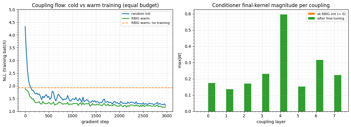
At an equal budget the warm flow is ahead the entire way — it opens near the random flow’s final loss and settles at a better optimum — and the bar chart tells the mechanistic story: the conditioner kernels lift off zero during training (right). The flow transitions from “diagonal RBIG marginal” to “true coupling” exactly as the kernels switch on. (The expressive coupling flow can reach a good fit from a random start too, but it needs more steps and lands slightly worse here — warm-start buys both speed and a better optimum, as it did for the diagonal flow in notebook 01.)

4. The learned densities¶

gx, gy = np.meshgrid(np.linspace(-2.5, 2.5, 120), np.linspace(-2.5, 2.5, 120))
grid = jnp.asarray(np.column_stack([gx.ravel(), gy.ravel()]))
fig, axes = plt.subplots(1, 3, figsize=(14.5, 4.6))
axes[0].scatter(X[:, 0], X[:, 1], color="tab:blue", **SCATTER_KW)
axes[0].set(title="data", xlabel="$x_0$", ylabel="$x_1$")
for ax, model, t in [(axes[1], cold, "random init"),
                     (axes[2], warm, "RBIG warm")]:
    lp = np.asarray(jax.vmap(model.log_prob)(grid)).reshape(gx.shape)
    ax.contourf(gx, gy, np.exp(lp), levels=18, cmap="viridis")
    ax.scatter(X[:, 0], X[:, 1], s=3, color="white", alpha=0.2)
    ax.set(title=f"{t}\nlog p = {logp(model):.2f}", xlabel="$x_0$")
for ax in axes:
    ax.set_aspect("equal"); style_ax(ax)
fig.suptitle("Warm-started coupling: better fit at an equal training budget", y=1.02)
fig.tight_layout()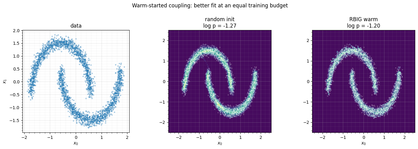

Recap¶

start	init log p	conditioner kernel	training (3000 steps)	final log p
random coupling	-4.3	random noise	lr $3\times10^{-3}$	$\approx -1.28$
RBIG warm	-1.9	exactly 0 (= diagonal)	lr 10^-3	$\approx -1.20$ (better)

fit_rbig_coupling warm-starts a coupling flow by the zero-kernel contract: conditioners emit constants, so each coupling is a diagonal RBIG marginal at init.
Gradient training drives the kernels off zero — the couplings switch from diagonal to genuinely conditional, the coupling↔diagonal equivalence breaking as it trains.
At an equal training budget the warm start is ahead the whole way and lands at a better optimum — buying both speed and quality, as it did for the diagonal flow in Part 4. (Coupling is the more expensive architecture, so it wants a real training budget — a few thousand steps — to converge.)

Next up. The zero-kernel contract showed empirically that a coupling can behave exactly like a diagonal marginal. 06 — Coupling ↔ diagonal equivalence makes that a precise, numerically verified statement: a zero-conditioner coupling and a diagonal flow are the same map at init, and training is what breaks the equivalence.

References¶

Kingma, D. P., & Dhariwal, P. (2018). Glow: Generative Flow with Invertible 1x1 Convolutions. Advances in Neural Information Processing Systems (NeurIPS).