Density destructors - Research Notebook

04 — Density destructors¶

Notebooks 00–03 assembled all the parts: an invertible map carries a density (change of variables), maps compose with additive log-dets, the two directions trade off, and $\mathcal{N}(0, I)$ is the natural target. Now we name the object those parts describe — a density destructor — and build one explicitly.

What you will see

The density-destructor definition (Inouye & Ravikumar, 2018) and how it unifies “normalizing flow”, “Gaussianization”, and “density destructor”.
The canonical recipe: alternate a marginal Gaussianization (elementwise nonlinearity) with a rotation, because neither move alone suffices.
Two-moons morphing into $\mathcal{N}(0, I)$ across rbig’s iterations — the “intuition picture” for the whole method.
Running the destructor backward to generate moon-shaped samples from Gaussian noise.

import warnings

warnings.filterwarnings("ignore")

import matplotlib.pyplot as plt
import numpy as np
from sklearn.datasets import make_moons

import rbig
from _style import style_ax

rng = np.random.default_rng(4)

X, _ = make_moons(6000, noise=0.05, random_state=0)
X = (X - X.mean(0)) / X.std(0)  # standardise so the base is N(0, I)

1. What is a density destructor?¶

Inouye & Ravikumar Inouye & Ravikumar (2018) define a density destructor as an invertible map $T:\mathbb{R}^d\to\mathbb{R}^d$ that turns the data distribution into a fixed, structureless base — here the standard Gaussian:

T_\# p_X = \mathcal{N}(0, I) \qquad\Longleftrightarrow\qquad z = T(x) \sim \mathcal{N}(0, I)\ \text{ when } x \sim p_X.

((1))

It “destroys” the density: everything that made $p_X$ structured — skew, heavy tails, multi-modality, dependence between coordinates — is removed, leaving isotropic Gaussian noise. This is the same object the rest of the field calls by other names, and each earlier notebook is one of its capabilities:

once you have a destructor $T$	you get…	from notebook
$\log p_X(x) = \log\mathcal{N}(T(x)) + \log\lvert\det J_T\rvert$	exact density	00, 01
$x = T^{-1}(z),\ z\sim\mathcal{N}(0,I)$	a generator	02
$\mathrm{TC}(T(x)) = 0$ , negentropy $=0$	independent, IT-friendly coords	03

“Normalizing flow” (ML), “Gaussianization” (signal processing), and “density destructor” (Inouye–Ravikumar) are three names for this one map. The whole curriculum is about building good ones.

2. The canonical recipe: nonlinearity + rotation¶

How do we construct $T$ for a tangled distribution like two-moons? The classic answer — Gaussianization Chen & Gopinath (2000) via Rotation-Based Iterative Gaussianization (RBIG) Laparra et al. (2011) — alternates two moves that each fix what the other cannot:

Marginal Gaussianization — apply $z_i = \Phi^{-1}(F_i(x_i))$ to each coordinate independently. This makes every axis standard normal, but being elementwise it cannot touch the dependence between axes.
Rotation — apply an orthogonal $Q$ . This is free ( $\log|\det| = 0$ , notebook 01) and mixes the axes, exposing new non-Gaussian structure along fresh directions for the next marginal step.

Neither alone works: marginals-only leaves the moons’ dependence intact; rotations-only never fixes the marginal shapes. Watch one iteration.

mg = rbig.MarginalGaussianize().fit(X)
X_marg = mg.transform(X)                      # step 1: elementwise nonlinearity
rot = rbig.RandomRotation(random_state=0).fit(X_marg)
X_rot = rot.transform(X_marg)                 # step 2: rotation

fig, axes = plt.subplots(1, 3, figsize=(12, 4))
for ax, data, title in [
    (axes[0], X, "data $x$ (two-moons)"),
    (axes[1], X_marg, "after marginal Gaussianization\n(axes ~N(0,1), shape remains)"),
    (axes[2], X_rot, "after rotation\n(structure remixed across axes)"),
]:
    ax.scatter(data[:3000, 0], data[:3000, 1], s=5, alpha=0.22, edgecolors="none")
    ax.set(title=title, xlim=(-4, 4), ylim=(-4, 4), xlabel="$z_1$", ylabel="$z_2$")
    ax.set_aspect("equal")
    style_ax(ax)
fig.tight_layout()

print("per-axis std after marginal step:", X_marg.std(0).round(3),
      "(each axis standardised)")
print("the moon shape survives the marginal step — only the rotation can remix it")

per-axis std after marginal step: [1. 1.] (each axis standardised)
the moon shape survives the marginal step — only the rotation can remix it

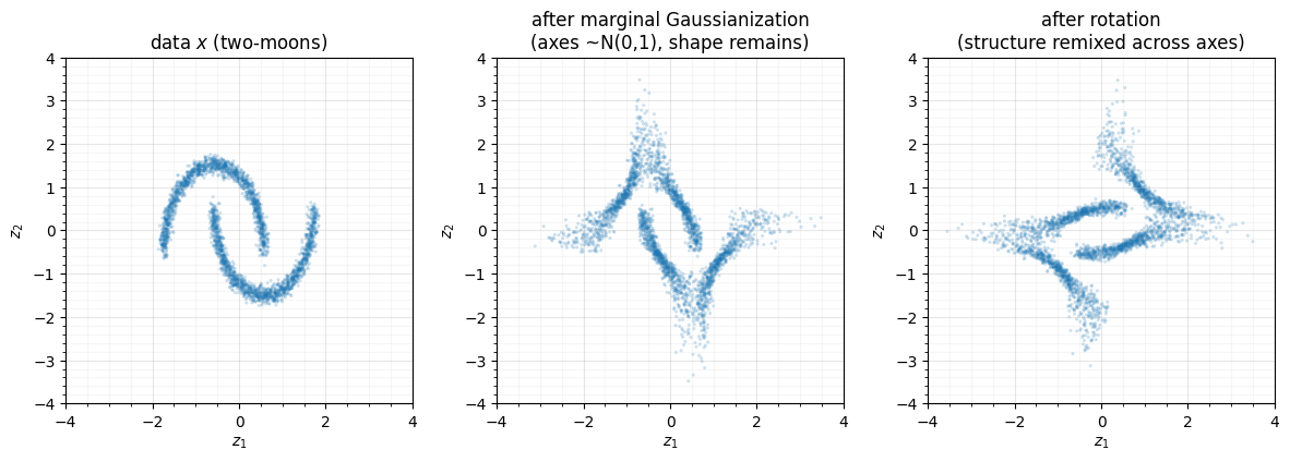
After step 1 each axis is individually standard-normal, yet the crescent shape is clearly still there — proof that elementwise maps cannot remove dependence. Step 2 rotates that structure onto new axes, where it again looks non-Gaussian per coordinate — so the next marginal step has something to bite on. One RBIGLayer in rbig is exactly this (marginal, rotation) pair.

3. Iterate to convergence — the intuition picture¶

Stack many (marginal, rotation) layers and the distribution is ground down toward $\mathcal{N}(0, I)$ . rbig.AnnealedRBIG is precisely this iterated destructor; we fit it and snapshot the data after $0, 3, 12,$ and all layers.

model = rbig.AnnealedRBIG(n_layers=100, rotation="random", random_state=0)
model.fit(X)


def through_layers(k):
    state = X
    for layer in model.layers_[:k]:
        state = layer.transform(state)
    return state


n_total = len(model.layers_)
fig, axes = plt.subplots(1, 4, figsize=(13, 3.6))
for ax, k in zip(axes, [0, 3, 12, n_total]):
    d = through_layers(k)
    ax.scatter(d[:3000, 0], d[:3000, 1], s=4, alpha=0.2, edgecolors="none")
    label = "data" if k == 0 else f"{k} layers"
    ax.set(title=label, xlim=(-4, 4), ylim=(-4, 4))
    ax.set_aspect("equal")
    style_ax(ax)
fig.suptitle(f"Two-moons → N(0, I): a density destructor at work "
             f"({n_total} RBIG layers)", y=1.02)
fig.tight_layout()
print(f"fitted {n_total} layers; final pushforward std = "
      f"{through_layers(n_total).std(0).round(3)}")

fitted 100 layers; final pushforward std = [1. 1.]

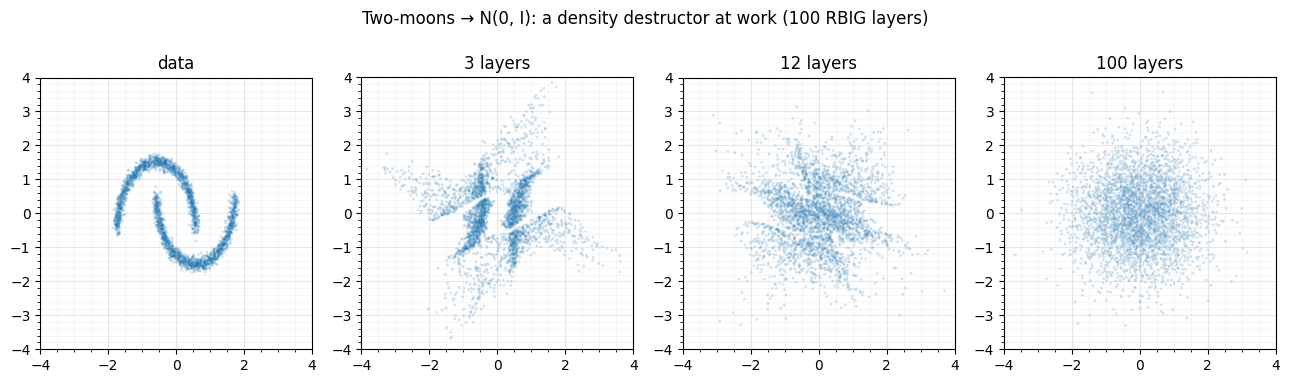
The crescents are progressively destroyed: by the last layer the data is an isotropic Gaussian blob with unit per-axis variance. That sequence is Gaussianization — iterated whitening-plus-nonlinearity grinding structure away. (How many layers are “enough” is a convergence question we quantify with diagnostics in notebook 06.)

4. Run it backward to generate¶

Because a density destructor is invertible, $T^{-1}$ is a generator: draw $z \sim \mathcal{N}(0, I)$ and push it back through the inverted layers to get data-shaped samples. rbig does this with model.sample, which internally inverts each marginal layer (the bisection/root-find of notebook 02) and transposes each rotation.

samples = np.asarray(model.sample(4000, random_state=1))

fig, axes = plt.subplots(1, 2, figsize=(9.5, 4.6), sharex=True, sharey=True)
axes[0].scatter(X[:3000, 0], X[:3000, 1], s=5, alpha=0.25, edgecolors="none")
axes[0].set(title="real data $x \\sim p_X$")
axes[1].scatter(samples[:3000, 0], samples[:3000, 1], s=5, alpha=0.25,
                edgecolors="none", color="tab:green")
axes[1].set(title=r"samples $x = T^{-1}(z),\ z\sim\mathcal{N}(0,I)$")
for ax in axes:
    ax.set(xlim=(-3, 3), ylim=(-3, 3), xlabel="$x_1$", ylabel="$x_2$")
    ax.set_aspect("equal")
    style_ax(ax)
fig.tight_layout()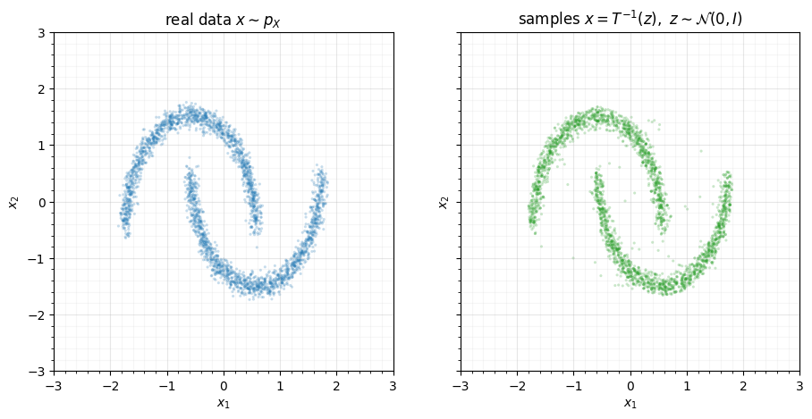

The same map, read in reverse, turns Gaussian noise back into two moons. A good density destructor is therefore simultaneously a density estimator (forward) and a generative model (inverse) — one object, both jobs.

Recap¶

concept	statement	in code
density destructor	invertible $T$ with $T_\# p_X = \mathcal{N}(0,I)$	`rbig.AnnealedRBIG`
one RBIG layer	marginal Gaussianization ∘ rotation	`MarginalGaussianize` + `RandomRotation`
why both moves	marginals fix axes; rotations remix dependence	§2 three-panel
iterate	structure ground down to $\mathcal{N}(0,I)$	`model.layers_` snapshots
generate	run $T^{-1}$ on Gaussian draws	`model.sample`

Next up. Iterating $\Phi^{-1}\circ F$ hundreds of times is a numerical minefield — CDFs hit 0 and 1, $\Phi^{-1}$ blows up, log-dets must not drift. 05 — Numerical mechanics covers the jitter, clamping, and float64 bookkeeping that keep a deep destructor stable.

References¶

Inouye, D. I., & Ravikumar, P. (2018). Deep Density Destructors. International Conference on Machine Learning (ICML).
Chen, S. S., & Gopinath, R. A. (2000). Gaussianization. Advances in Neural Information Processing Systems (NeurIPS).
Laparra, V., Camps-Valls, G., & Malo, J. (2011). Iterative Gaussianization: From ICA to Random Rotations. IEEE Transactions on Neural Networks, 22(4), 537–549. 10.1109/TNN.2011.2106511
Meng, C., Song, Y., Song, J., & Ermon, S. (2020). Gaussianization Flows. International Conference on Artificial Intelligence and Statistics (AISTATS).