Why a standard Gaussian?
Maximum entropy, separability, and trivial primitives — the three reasons N(0, I) is the target
03 — Why a standard Gaussian?
Every notebook so far has mapped data to a standard Gaussian without questioning the destination. Why not a uniform, a Laplace, a heavy-tailed base? The choice is not arbitrary — earns its place through three properties, and each one buys Gaussianization something concrete.
What you will see
- Maximum entropy: at a fixed mean and covariance, the Gaussian is the
least committal distribution — highest differential entropy — so
rbig.negentropymeasures “distance from Gaussian”. - Separability: , so once we
reach it the coordinates are independent —
rbig.total_correlationcollapses to 0. - Trivial primitives: its sampler is one line, its log-density is a squared norm, and its score is simply .
import warnings

warnings.filterwarnings("ignore")

import jax
import jax.numpy as jnp
import jax.random as jr
import matplotlib.pyplot as plt
import numpy as np

import rbig
from _style import style_ax

jax.config.update("jax_enable_x64", True)
rng = np.random.default_rng(3)
1. Maximum entropy at fixed covariance
Among all distributions on with a given mean and covariance Σ, the Gaussian has the largest differential entropy Jaynes (1957)Cover & Thomas (2006):
In words: fixing the first two moments, the Gaussian assumes the least about everything else. That makes it the honest target — Gaussianizing says “I have captured the mean and covariance structure; what remains is structureless noise.” The gap between any distribution’s entropy and the Gaussian with the same covariance is the negentropy , with equality iff is Gaussian. Let’s see the ordering on several unit-variance distributions.
# Unit-variance versions of four distributions + their analytic entropies (nats).
b_lap = 1 / np.sqrt(2)                 # Laplace scale for unit variance
s_log = np.sqrt(3) / np.pi             # Logistic scale for unit variance
a_uni = np.sqrt(3)                     # Uniform half-width for unit variance
samplers = {
    "Gaussian": (lambda n: rng.standard_normal(n), 0.5 * np.log(2 * np.pi * np.e)),
    "Logistic": (lambda n: rng.logistic(0, s_log, n), np.log(s_log) + 2),
    "Laplace": (lambda n: rng.laplace(0, b_lap, n), 1 + np.log(2 * b_lap)),
    "Uniform": (lambda n: rng.uniform(-a_uni, a_uni, n), np.log(2 * a_uni)),
}

colors = ["tab:red", "tab:orange", "tab:green", "tab:blue"]
names = list(samplers)
H_analytic = np.array([samplers[k][1] for k in names])
J_analytic = H_analytic[0] - H_analytic  # negentropy vs the unit-variance Gaussian

# Corroborate the negentropy with rbig (a difference of entropies, so the
# estimator's constant bias cancels — unlike a raw entropy estimate).
J_rbig = np.array([
    float(rbig.negentropy(samplers[k][0](50_000)[:, None])[0]) for k in names
])

fig, axes = plt.subplots(1, 2, figsize=(11, 4.2))

bars = axes[0].bar(names, H_analytic, color=colors)
axes[0].axhline(H_analytic[0], color="tab:red", ls="--", lw=1,
                label="Gaussian entropy (the max)")
axes[0].bar_label(bars, fmt="%.3f", padding=3)
axes[0].set(ylabel="differential entropy (nats)", ylim=(1.1, 1.48),
            title="Gaussian has the most entropy\n(at fixed unit variance)")
axes[0].legend(loc="lower left", fontsize=8)
style_ax(axes[0])

bars = axes[1].bar(names, J_analytic, color=colors, alpha=0.55)
axes[1].plot(names, J_rbig, "ko", ms=8, label="rbig.negentropy estimate")
axes[1].bar_label(bars, fmt="%.3f", padding=3)
axes[1].set(ylabel="negentropy $J$ (nats)",
            title=r"negentropy $J = H_{\mathcal{N}} - H \geq 0$"
                  "\n(zero iff Gaussian)")
axes[1].legend(loc="upper left", fontsize=8)
style_ax(axes[1])
fig.tight_layout()

print("negentropy J = H_Gaussian - H (>= 0, zero iff Gaussian):")
for k, Ja, Jr in zip(names, J_analytic, J_rbig):
    print(f"  {k:9s}: analytic J = {Ja:.4f},  rbig.negentropy = {Jr:.4f} nats")
negentropy J = H_Gaussian - H (>= 0, zero iff Gaussian):
Gaussian : analytic J = 0.0000, rbig.negentropy = 0.0003 nats
Logistic : analytic J = 0.0144, rbig.negentropy = 0.0138 nats
Laplace : analytic J = 0.0724, rbig.negentropy = 0.0735 nats
Uniform : analytic J = 0.1765, rbig.negentropy = 0.1434 nats
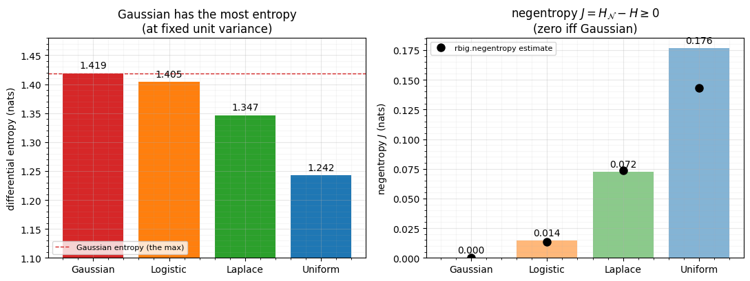
The Gaussian bar is the tallest, and rbig’s estimator (black dots) tracks the
analytic values. Every other distribution has positive negentropy — a
quantitative “how non-Gaussian am I”. Driving that gap to zero is
Gaussianization, which is why rbig.negentropy doubles as a convergence signal
(we use it that way in Part 3).
2. Separability: 
The standard Gaussian is special among Gaussians: with identity covariance it factorises into independent unit-variance coordinates,
Independent coordinates means zero total correlation Watanabe (1960)
— no multi-information left. So
Gaussianization is really two jobs in one: remove dependence and normalise
margins. We can watch the dependence disappear: take a strongly correlated 2D
Gaussian, whiten it to , and measure TC with rbig before
and after.
C = np.array([[1.0, 0.85], [0.85, 1.0]])
X = rng.standard_normal((20000, 2)) @ np.linalg.cholesky(C).T
Xw = rbig.PCARotation(whiten=True).fit(X).transform(X)

tc_before = rbig.total_correlation(X)
tc_after = rbig.total_correlation(Xw)
print(f"total correlation before whitening = {tc_before:.4f} nats")
print(f"total correlation after  whitening = {tc_after:.4f} nats  (~0)")

fig, axes = plt.subplots(1, 2, figsize=(10, 4.6), sharex=True, sharey=True)
for ax, data, title, tc in [
    (axes[0], X, "correlated Gaussian", tc_before),
    (axes[1], Xw, r"after whitening $\to \mathcal{N}(0, I)$", tc_after),
]:
    ax.scatter(data[:3000, 0], data[:3000, 1], s=6, alpha=0.25, edgecolors="none")
    ax.set(title=f"{title}\nTC = {tc:.3f} nats", xlabel="$z_1$", ylabel="$z_2$",
           xlim=(-4, 4), ylim=(-4, 4))
    ax.set_aspect("equal")
    style_ax(ax)
fig.tight_layout()
total correlation before whitening = 0.6517 nats
total correlation after whitening = -0.0015 nats (~0)
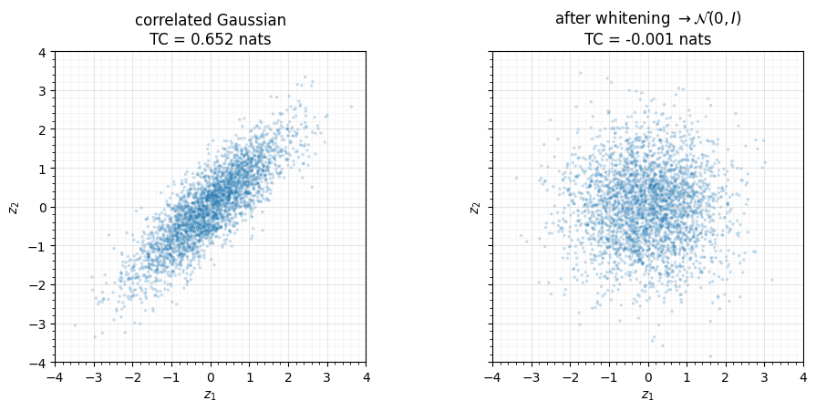
The left cloud leans along the diagonal — knowing tells you a lot about (TC nats). The right cloud is isotropic; the coordinates are independent and TC has collapsed to ~0. After reaching , information-theoretic quantities decompose per coordinate, which is exactly what makes Gaussianized representations so convenient for entropy and mutual-information estimation (Part 14).
3. Trivial primitives
Finally, is the computationally easiest base a flow could sit on. Three things every flow needs from its base are all one-liners:
- Sampling: is
jax.random.normal— no MCMC, no rejection. - Log-density: — just a squared norm.
- Score: — a linear vector field pointing at the origin.
The score being exactly is worth dwelling on: it is what makes the base
trivial for score-based and diffusion methods Song & Ermon (2019)
(Part 9). Let’s confirm it by autodiff, and read the base straight off a
gauss_flows flow.
import gauss_flows as gf

flow = gf.gaussianization_flow(jr.key(0), n_dims=2, n_layers=4, n_components=8)
base = flow.base_dist  # the N(0, I) every Gaussianization flow targets

z = jnp.asarray(rng.standard_normal(2))
score = jax.grad(base.log_prob)(z)   # d/dz log p(z)
print(f"z                      = {np.asarray(z)}")
print(f"score grad log p(z)    = {np.asarray(score)}")
print(f"-z                     = {np.asarray(-z)}")
print(f"score == -z ?            {bool(jnp.allclose(score, -z, atol=1e-6))}")

# Visualise the score field: it points straight at the origin everywhere.
gx, gy = np.meshgrid(np.linspace(-2.5, 2.5, 13), np.linspace(-2.5, 2.5, 13))
pts = np.stack([gx.ravel(), gy.ravel()], 1)
S = jax.vmap(jax.grad(base.log_prob))(jnp.asarray(pts))
S = np.asarray(S)

fig, ax = plt.subplots(figsize=(5.2, 5))
ax.quiver(pts[:, 0], pts[:, 1], S[:, 0], S[:, 1], color="tab:purple",
          alpha=0.8, scale=30)
ax.plot(0, 0, "k*", ms=12)
ax.set(title=r"score of $\mathcal{N}(0, I)$ is $-z$ (linear field)",
       xlabel="$z_1$", ylabel="$z_2$")
ax.set_aspect("equal")
style_ax(ax)
fig.tight_layout()
z = [-0.12028701 1.32257788]
score grad log p(z) = [ 0.12028701 -1.32257788]
-z = [ 0.12028701 -1.32257788]
score == -z ? True
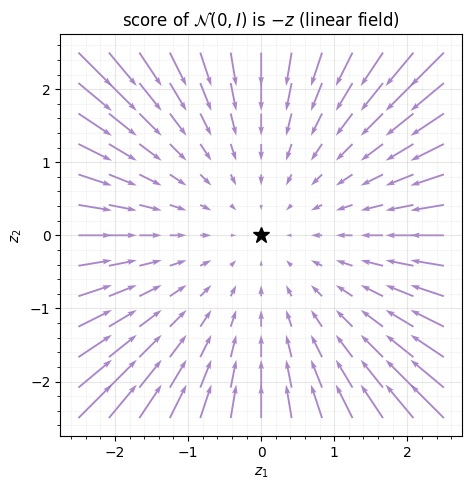
Autodiff confirms , and the quiver shows the field is a
clean linear pull toward the origin — no curvature, no surprises. Cheap
sampling, a squared-norm density, and a linear score together make
the base that keeps flow.log_prob and flow.sample cheap
in notebook 02.
Recap
| property | statement | what it buys | package |
|---|---|---|---|
| max entropy | Gaussian maximises at fixed Σ | negentropy = “non-Gaussianity” | rbig.negentropy |
| separability | TC ; IT decomposes per-coord | rbig.total_correlation | |
| trivial sampler | jax.random.normal | cheap generation | flow.sample |
| trivial density | cheap log_prob base term | flow.base_dist.log_prob | |
| trivial score | linear field for diffusion/score | jax.grad(base.log_prob) |
Next up. With the target justified, we name the object we have been building. 04 — Density destructors introduces the Inouye–Ravikumar framing — Gaussianization as iterated whitening plus an elementwise nonlinearity — and the picture that ties the whole method together.
- Jaynes, E. T. (1957). Information Theory and Statistical Mechanics. Physical Review, 106(4), 620–630. 10.1103/PhysRev.106.620
- Cover, T. M., & Thomas, J. A. (2006). Elements of Information Theory (2nd ed.). Wiley-Interscience.
- Watanabe, S. (1960). Information Theoretical Analysis of Multivariate Correlation. IBM Journal of Research and Development, 4(1), 66–82. 10.1147/rd.41.0066
- Song, Y., & Ermon, S. (2019). Generative Modeling by Estimating Gradients of the Data Distribution. Advances in Neural Information Processing Systems (NeurIPS).