Forward vs. inverse parameterisation

02 — Forward vs. inverse parameterisation¶

A normalizing flow is a bijection $T$ , so it can be run in either direction. That sounds symmetric, but it almost never is: one direction is a closed-form expression and the other needs an iterative solve. Which direction you make cheap decides whether your flow is good at density estimation or at sampling.

What you will see

The two operations a flow supports — log_prob (forward) and sample (inverse) — and which direction each needs.
A mixture-CDF whose forward $F(x)$ is one closed-form line but whose inverse $F^{-1}(u)$ we solve with optimistix.root_find (bisection).
A real gauss_flows flow where log_prob is ~39× faster than sample, and the flowjax.Invert parameterisation choice (the MAF ↔ IAF duality).

import warnings

warnings.filterwarnings("ignore")

import time

import equinox as eqx
import jax
import jax.numpy as jnp
import jax.random as jr
import jax.scipy.stats as jstats
import matplotlib.pyplot as plt
import numpy as np
import optimistix as optx

from _style import style_ax

jax.config.update("jax_enable_x64", True)
rng = np.random.default_rng(2)

1. A flow runs both ways¶

Let $z = T(x)$ map data to a standard-Gaussian latent. The two things we ever ask of a flow use opposite directions:

operation	direction	needs	used for
`log_prob(x)`	forward $x \to z$	$T(x)$ and $\log\lvert\det J_T(x)\rvert$	density estimation, MLE training
`sample()`	inverse $z \to x$	$T^{-1}(z)$ , $z\sim\mathcal{N}(0,I)$	generation, simulation

Both are always possible (that’s what “bijection” means), but their cost and their differentiability can differ sharply. The culprit is the marginal transform.

2. Analytic forward, iterative inverse — with `optimistix`¶

The atom of Gaussianization is the per-coordinate map $z = \Phi^{-1}(F(x))$ , where $F$ is a mixture-of-Gaussians CDF,

F(x) = \sum_{k} w_k\,\Phi\!\Big(\frac{x-\mu_k}{\sigma_k}\Big).

((1))

Forward ( $x \to u = F(x)$ ) is one closed-form sum. Inverse ( $u \to x = F^{-1}(u)$ ) has no closed form, so we frame it as a root-find: solve $g(x) = F(x) - u = 0$ . We hand that to optimistix Kidger (2021) — the same solver library gauss_flows depends on — using its bracketing Bisection solver, which is bullet-proof because $F$ is monotone.

w = jnp.array([0.4, 0.35, 0.25])
mu = jnp.array([-1.5, 0.3, 2.0])
sd = jnp.array([0.4, 0.6, 0.5])


def F(x):  # mixture-of-Gaussians CDF (forward), closed form
    return jnp.sum(w * jstats.norm.cdf(x, mu, sd))


F_v = jax.vmap(F)

_solver = optx.Bisection(rtol=1e-10, atol=1e-12)


def invF(u, max_steps=200):
    """x = F^{-1}(u) via optimistix bisection on g(x) = F(x) - u."""
    sol = optx.root_find(
        lambda x, args: F(x) - args, _solver, 0.0, args=u,
        options=dict(lower=-12.0, upper=12.0), max_steps=max_steps, throw=False,
    )
    return sol.value


# Round-trip: push real samples forward, then recover them with the solver.
x_true = jnp.asarray(rng.normal(0.3, 1.2, size=400))
u_targets = F_v(x_true)
x_rec = jax.vmap(invF)(u_targets)
print("forward F(x): closed form, one evaluation")
print(f"inverse F^-1(u) via optimistix: max|x - x_rec| = "
      f"{float(jnp.max(jnp.abs(x_true - x_rec))):.2e}")

# Accuracy vs. solver budget: bisection error falls geometrically (~2^-n).
steps = np.arange(1, 46)
u0 = 0.7
err_vs_steps = np.array(
    [abs(float(F(invF(u0, max_steps=int(k))) - u0)) for k in steps]
)

forward F(x): closed form, one evaluation
inverse F^-1(u) via optimistix: max|x - x_rec| = 1.63e-10

fig, axes = plt.subplots(1, 2, figsize=(11, 4.2))

xg = jnp.linspace(-4, 4, 500)
axes[0].plot(xg, F_v(xg), color="tab:blue", lw=2, label="$F(x)$ (forward, analytic)")
for u in [0.2, 0.5, 0.8]:
    xr = float(invF(jnp.asarray(u)))
    axes[0].hlines(u, -4, xr, color="tab:orange", lw=1, ls=":")
    axes[0].vlines(xr, 0, u, color="tab:orange", lw=1, ls=":")
    axes[0].plot(xr, u, "o", color="tab:orange", ms=6)
axes[0].set(title="forward is a lookup; inverse is a root-find",
            xlabel="x", ylabel="$u = F(x)$")
axes[0].legend(loc="upper left")
style_ax(axes[0])

axes[1].semilogy(steps, err_vs_steps, "-o", color="tab:red", ms=3)
axes[1].axhline(1e-12, color="k", lw=0.8, ls="--", label=r"$\approx$ float64 floor")
axes[1].set(title=r"optimistix bisection: error $\sim 2^{-n}$",
            xlabel="solver max_steps", ylabel=r"residual $|F(x_\star) - u|$")
axes[1].legend()
style_ax(axes[1])
fig.tight_layout()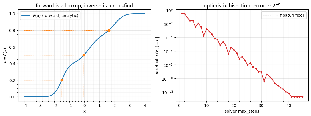

Left: inverting $F$ means reading the curve right-to-left — there is no formula, so optimistix hunts for the $x$ that lands on each target $u$ . Right: the residual falls geometrically with the solver budget, hitting the float64 floor in ~40 steps. Accurate and robust — but it is a loop. How to differentiate that loop (and why naively unrolling it fails) is its own story, told in Part 1, notebook 03 when we train a mixture-CDF.

3. The asymmetry on a real flow¶

gauss_flows builds its marginal layers from exactly this mixture-CDF, so a whole flow inherits the asymmetry: log_prob runs the analytic forward maps, while sample runs the bisection inverse inside every marginal layer. We time both on the same flow (JIT-compiled and warmed up for a fair race).

import gauss_flows as gf

key = jr.key(0)
flow = gf.gaussianization_flow(key, n_dims=2, n_layers=6, n_components=8)
X = jnp.asarray(rng.standard_normal((5000, 2)))


@eqx.filter_jit
def logp(f, x):
    return f.log_prob(x)


@eqx.filter_jit
def samp(f, k):
    return f.sample(k, (5000,))


logp(flow, X).block_until_ready()           # warmup (compile)
samp(flow, key).block_until_ready()

t = time.perf_counter()
for _ in range(5):
    logp(flow, X).block_until_ready()
t_lp = (time.perf_counter() - t) / 5

t = time.perf_counter()
for i in range(5):
    samp(flow, jr.fold_in(key, i)).block_until_ready()
t_s = (time.perf_counter() - t) / 5

print(f"log_prob (forward, analytic)  : {t_lp * 1e3:6.2f} ms / 5000 pts")
print(f"sample   (inverse, bisection) : {t_s * 1e3:6.2f} ms / 5000 pts")
print(f"sample is {t_s / t_lp:.0f}x more expensive than log_prob")

log_prob (forward, analytic)  :  19.54 ms / 5000 pts
sample   (inverse, bisection) : 764.82 ms / 5000 pts
sample is 39x more expensive than log_prob

fig, ax = plt.subplots(figsize=(6.2, 4))
bars = ax.bar(["log_prob\n(forward)", "sample\n(inverse)"],
              [t_lp * 1e3, t_s * 1e3], color=["tab:blue", "tab:orange"])
ax.bar_label(bars, fmt="%.1f ms", padding=3)
ax.set(ylabel="wall-clock (ms / 5000 points)",
       title=f"Same flow, opposite directions: {t_s / t_lp:.0f}x gap")
style_ax(ax)
fig.tight_layout()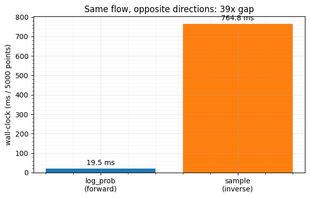

4. The parameterisation choice¶

The map $T$ and its inverse $T^{-1}$ describe the same flow — but we choose which one to store as the cheap, closed-form direction. Whatever we store cheaply, the other direction pays the iterative price.

Density-estimation flows call log_prob constantly. Store the forward map cheaply → fast training, slow sampling. This is what gauss_flows Gaussianization flows do, hence §3.
Sampling / variational flows call sample constantly. Store the inverse cheaply → fast sampling, slow density.

In flowjax the switch is one wrapper, Invert, which swaps a bijector’s forward and inverse.

from flowjax.bijections import Invert

b = gf.MixtureGaussianCDF(n_components=8, shape=(2,))
x = jnp.array([0.4, -0.7])
bi = Invert(b)  # forward and inverse swapped
print("Invert(b).transform == b.inverse :",
      bool(jnp.allclose(bi.transform(x), b.inverse(x))))
print("=> 'forward' and 'inverse' are a labelling choice, not a fixed property.")

Invert(b).transform == b.inverse : True
=> 'forward' and 'inverse' are a labelling choice, not a fixed property.

Recap¶

concept	takeaway	in code
two directions	forward for density, inverse for sampling	`flow.log_prob` / `flow.sample`
mixture-CDF inverse	a monotone root-find	`optimistix.root_find` + `Bisection`
measured asymmetry	`sample` ≈ 39× `log_prob` for Gaussianization	timed, JIT-warmed
parameterisation	store the cheap direction; `Invert` swaps it	`flowjax.bijections.Invert`
differentiating the inverse	unrolling / one-step / adjoint	Part 1, nb 03

Next up. We have been mapping to a standard Gaussian without asking why that target. 03 — Why a standard Gaussian? shows the three properties — maximum entropy, separability, trivial primitives — that make $\mathcal{N}(0, I)$ the natural destination.

References¶

Kidger, P. (2021). On Neural Differential Equations [Phdthesis]. University of Oxford.
Papamakarios, G., Pavlakou, T., & Murray, I. (2017). Masked Autoregressive Flow for Density Estimation. Advances in Neural Information Processing Systems (NeurIPS).
Kingma, D. P., Salimans, T., Jozefowicz, R., Chen, X., Sutskever, I., & Welling, M. (2016). Improving Variational Inference with Inverse Autoregressive Flow. Advances in Neural Information Processing Systems (NeurIPS).
Dinh, L., Sohl-Dickstein, J., & Bengio, S. (2017). Density Estimation using Real NVP. International Conference on Learning Representations (ICLR).

Forward vs. inverse parameterisation

02 — Forward vs. inverse parameterisation¶

1. A flow runs both ways¶

2. Analytic forward, iterative inverse — with optimistix¶

3. The asymmetry on a real flow¶

4. The parameterisation choice¶

Recap¶

2. Analytic forward, iterative inverse — with `optimistix`¶