Inversion strategies - Research Notebook

04 — Inversion strategies¶

Notebooks 01–03 all reduced “invert the marginal” to the same problem: solve the monotone equation $F(x) = u$ for $x$ . This closing notebook of Part 1 is about how to solve it well — the trade-off between bisection and Newton, the safeguarded hybrid that production solvers use, and how to run the solve on a whole batch at once.

What you will see

Bisection: bracketing, derivative-free, linearly convergent (one bit per step → ~50 steps for float64), and bullet-proof for monotone $F$ .
Newton: uses $F'$ (the density), quadratically convergent (~5 steps), but can overshoot or diverge in flat tails.
The safeguarded Newton hybrid — Newton when it stays in the bracket, else bisect — fast and robust.
Differentiating the inverse four ways (unroll-bisection, unroll-Newton, one-step, adjoint) — the gradient depends on the solver, and gauss_flows’ unrolled bisection returns zero.
Vectorising the root-find across a batch with jax.vmap.

import warnings

warnings.filterwarnings("ignore")

import time

import gauss_flows as gf
import jax
import jax.numpy as jnp
import jax.scipy.stats as jstats
import matplotlib.pyplot as plt
import numpy as np
import optimistix as optx

from _style import style_ax

jax.config.update("jax_enable_x64", True)
rng = np.random.default_rng(14)

# A 3-component mixture CDF F and its density F' (= forward derivative).
w = jnp.array([0.4, 0.35, 0.25])
mu = jnp.array([-1.5, 0.3, 2.0])
sd = jnp.array([0.4, 0.6, 0.5])


def F(x):
    return jnp.sum(w * jstats.norm.cdf(x, mu, sd))


def Fp(x):  # F'(x): the mixture density, Newton's slope
    return jnp.sum(w * jstats.norm.pdf(x, mu, sd))

1. Bisection vs. Newton¶

Both solve $F(x) = u$ for a monotone $F$ , but they trade robustness against speed.

Bisection keeps a bracket $[\text{lo}, \text{hi}]$ straddling the root and halves it each step. The error falls like $2^{-n}$ — linear convergence — so reaching float64 takes ~50 steps. It needs no derivative and cannot fail for a monotone $F$ .
Newton iterates $x_{n+1} = x_n - (F(x_n) - u)/F'(x_n)$ . Near the root the error roughly squares each step — quadratic convergence, ~5 steps — but it needs $F'$ and, with no bracket, can overshoot into a flat tail where $F'\approx 0$ and diverge. We record the per-iteration error of each.

def bisection(u, n_iter=55):
    lo, hi, errs = -12.0, 12.0, []
    for _ in range(n_iter):
        mid = 0.5 * (lo + hi)
        errs.append(abs(float(F(mid) - u)))
        if F(mid) < u:
            lo = mid
        else:
            hi = mid
    return np.array(errs)


def newton(u, x0=0.0, n_iter=12):
    x, errs = x0, []
    for _ in range(n_iter):
        errs.append(abs(float(F(x) - u)))
        x = x - (F(x) - u) / Fp(x)
    return np.array(errs)


u = 0.7
err_bis, err_newt = bisection(u), newton(u)
print(f"bisection: {len(err_bis)} steps to {err_bis[-1]:.1e}  (linear)")
print(f"newton:    reaches {err_newt[5]:.1e} in 5 steps        (quadratic)")

# Newton's fragility: from a far-tail start aiming at an extreme quantile.
err_newt_bad = newton(0.999, x0=-8.0, n_iter=8)
print(f"newton from a bad tail start: errors = "
      f"{[f'{e:.0e}' for e in err_newt_bad[:6]]}  -> diverges (nan)")

bisection: 55 steps to 1.1e-16  (linear)
newton:    reaches 1.1e-16 in 5 steps        (quadratic)
newton from a bad tail start: errors = ['1e+00', '1e-03', '1e+00', 'nan', 'nan', 'nan']  -> diverges (nan)

fig, axes = plt.subplots(1, 2, figsize=(11, 4.2))
axes[0].semilogy(range(1, len(err_bis) + 1), np.maximum(err_bis, 1e-17), "-o",
                 ms=3, color="tab:blue", label="bisection (linear)")
axes[0].semilogy(range(1, len(err_newt) + 1), np.maximum(err_newt, 1e-17), "-s",
                 ms=4, color="tab:green", label="Newton (quadratic)")
axes[0].set(title="convergence: Newton is far faster",
            xlabel="iteration", ylabel=r"residual $|F(x_n) - u|$")
axes[0].legend(); style_ax(axes[0])

steps_bad = np.arange(1, len(err_newt_bad) + 1)
finite = np.isfinite(err_newt_bad)
axes[1].semilogy(steps_bad[finite], np.maximum(err_newt_bad[finite], 1e-17), "-s",
                 ms=5, color="tab:red", label="plain Newton (diverges → nan)")
axes[1].axvspan(steps_bad[finite][-1], len(err_newt_bad), color="tab:red", alpha=0.08)
axes[1].set(title="...but Newton alone is fragile in the tails",
            xlabel="iteration", ylabel="residual")
axes[1].legend(); style_ax(axes[1])
fig.tight_layout()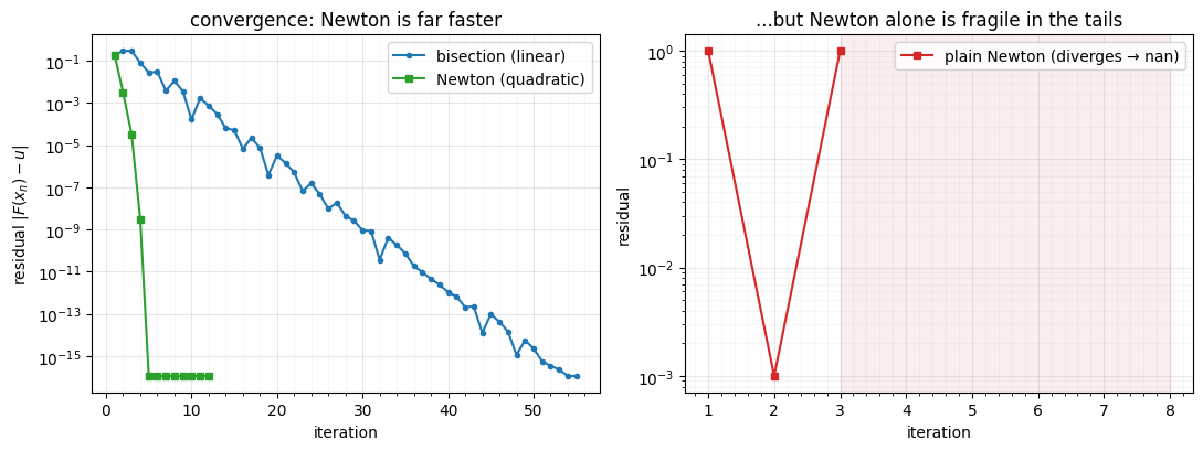

Left: Newton (green) reaches machine precision in ~5 steps where bisection (blue) needs ~50 — quadratic vs. linear. Right: starting Newton far out in the tail, the tiny $F'$ throws the iterate even further out and it blows up to nan. Bisection would simply have kept halving. We want Newton’s speed without its fragility.

2. The safeguarded hybrid¶

The standard fix (Brent-style Brent (1973)) keeps a bracket like bisection but tries a Newton step each iteration, accepting it only if it lands inside the bracket; otherwise it falls back to the bisection midpoint. This keeps the guaranteed convergence of bisection and the speed of Newton near the root — and it is essentially what robust library solvers do.

def safeguarded_newton(u, n_iter=60):
    lo, hi, x, errs = -12.0, 12.0, 0.0, []
    for _ in range(n_iter):
        errs.append(abs(float(F(x) - u)))
        lo, hi = (x, hi) if F(x) < u else (lo, x)   # tighten bracket
        step = x - (F(x) - u) / Fp(x)               # Newton proposal
        x = step if lo < step < hi else 0.5 * (lo + hi)  # accept or bisect
    return np.array(errs)


err_safe = safeguarded_newton(0.999)  # the same hard target that broke Newton
print(f"safeguarded Newton on the hard tail target: {err_safe[-1]:.1e}, "
      f"all finite = {bool(np.all(np.isfinite(err_safe)))}")

fig, ax = plt.subplots(figsize=(7, 4))
ax.semilogy(range(1, len(err_safe) + 1), np.maximum(err_safe, 1e-17), "-o", ms=3,
            color="tab:purple", label="safeguarded Newton")
ax.semilogy(range(1, len(err_bis) + 1), np.maximum(err_bis, 1e-17), "--", lw=1,
            color="tab:blue", label="bisection (for reference)")
ax.set(title="Safeguarded Newton: fast and robust (hard tail target)",
       xlabel="iteration", ylabel=r"residual $|F(x_n) - u|$")
ax.legend(); style_ax(ax)
fig.tight_layout()

safeguarded Newton on the hard tail target: 1.1e-16, all finite = True

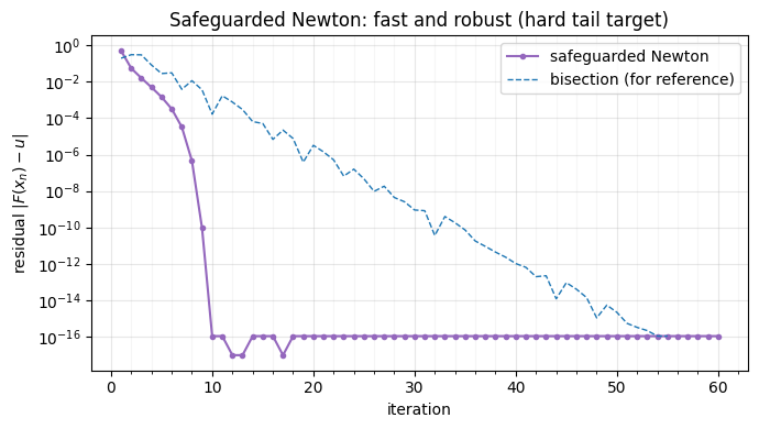
On the very target that sent plain Newton to nan, the safeguarded version stays finite and converges quickly — the bracket catches every bad Newton step. optimistix Kidger (2021) ships both primitives (optx.Bisection, optx.Newton) and composes them; gauss_flows uses the robust bracketing bisection by default (we saw its internals in notebook 03).

3. Differentiating the inverse¶

To train a flow through its sampling path we need to differentiate the inverse — $\partial x_\star/\partial u$ and $\partial x_\star/\partial\theta$ . Crucially, whether you get the right gradient depends on the solver. There are four options:

strategy	idea	pros	cons
unroll bisection	backprop the bracketing loop	trivial	wrong (zero) — the `where(F<u)` comparisons are piecewise constant
unroll Newton	backprop the smooth update	correct gradient; trivial	memory $O(\#\text{iters})$ — stores every iterate
one-step	detach the root, add one Newton step	exact; $O(1)$ memory; ~3 lines	needs $F'$ at $x_\star$
adjoint (implicit-fn thm)	differentiate $F(x_\star)=u$ directly	exact; $O(1)$ ; automatic in `optimistix`; scales to vector roots	a linear solve

The last three all compute the implicit-function gradient Blondel et al. (2022), which depends only on the solution:

\frac{\partial x_\star}{\partial u} = \frac{1}{F'(x_\star)}, \qquad \frac{\partial x_\star}{\partial \theta} = -\frac{\partial_\theta F(x_\star)}{F'(x_\star)} .

((1))

Unrolling instead differentiates the path to $x_\star$ — which is why it is correct for smooth Newton but useless for comparison-based bisection.

_isolver = optx.Bisection(rtol=1e-12, atol=1e-14)


def _solve(u):  # the converged root (used by one-step and adjoint)
    return optx.root_find(lambda x, a: F(x) - a, _isolver, 0.0, args=u,
                          options=dict(lower=-12.0, upper=12.0), max_steps=200,
                          throw=False).value


def inv_unroll_bisect(u, n=60):          # (1) unroll bisection -> zero grad
    lo, hi = -12.0, 12.0
    for _ in range(n):
        mid = 0.5 * (lo + hi)
        below = F(mid) < u
        lo = jnp.where(below, mid, lo)
        hi = jnp.where(below, hi, mid)
    return 0.5 * (lo + hi)


def inv_unroll_newton(u, n=30):          # (2) unroll Newton -> correct, O(n) memory
    x = 0.0
    for _ in range(n):
        x = x - (F(x) - u) / Fp(x)
    return x


def inv_onestep(u):                      # (3) detach + one Newton step -> exact, O(1)
    x_star = jax.lax.stop_gradient(_solve(u))
    return x_star - (F(x_star) - u) / Fp(x_star)


def inv_adjoint(u):                      # (4) optimistix ImplicitAdjoint -> exact, O(1)
    return _solve(u)


uu = jnp.linspace(0.03, 0.97, 40)
g_analytic = jax.vmap(lambda u: 1.0 / Fp(_solve(u)))(uu)
g_unroll_b = jax.vmap(jax.grad(inv_unroll_bisect))(uu)
g_unroll_n = jax.vmap(jax.grad(inv_unroll_newton))(uu)
g_onestep = jax.vmap(jax.grad(inv_onestep))(uu)
g_adjoint = jax.vmap(jax.grad(inv_adjoint))(uu)

amax = lambda g: float(jnp.max(jnp.abs(g - g_analytic)))
print(f"max |unroll-Newton - analytic| = {amax(g_unroll_n):.2e}   (correct)")
print(f"max |one-step     - analytic| = {amax(g_onestep):.2e}   (correct)")
print(f"max |adjoint      - analytic| = {amax(g_adjoint):.2e}   (correct)")
print(f"unroll-bisection grad range   = [{float(g_unroll_b.min()):.0e}, "
      f"{float(g_unroll_b.max()):.0e}]   <- zero (wrong)")

max |unroll-Newton - analytic| = 6.00e-12   (correct)
max |one-step     - analytic| = 0.00e+00   (correct)
max |adjoint      - analytic| = 3.55e-15   (correct)
unroll-bisection grad range   = [0e+00, 0e+00]   <- zero (wrong)

fig, ax = plt.subplots(figsize=(8, 4.4))
ax.plot(uu, g_analytic, "-", color="k", lw=2.5, label=r"analytic $1/F'(x_\star)$")
ax.plot(uu, g_adjoint, "o", color="tab:green", ms=6, label="adjoint (optimistix)")
ax.plot(uu, g_onestep, "s", color="tab:orange", ms=5, mfc="none", label="one-step Newton")
ax.plot(uu, g_unroll_n, "^", color="tab:purple", ms=5, mfc="none",
        label="unrolled Newton (O(n) mem)")
ax.plot(uu, g_unroll_b, "--", color="tab:red", lw=1.5, label="unrolled bisection (wrong: 0)")
ax.set(title=r"gradient of the inverse, $\partial x_\star/\partial u$, by strategy",
       xlabel="u", ylabel=r"$\partial x_\star / \partial u$")
ax.legend(fontsize=8); style_ax(ax)
fig.tight_layout()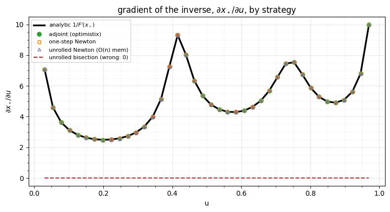

Three of the four land on the analytic curve; only unrolled bisection is flat at zero, because its iterates depend on the inputs solely through < comparisons. Unrolled Newton is correct — its update is smooth — but pays $O(\#\text{iters})$ memory, so the $O(1)$ one-step and adjoint methods win for deep flows. This trap is live: gauss_flows’ MixtureGaussianCDF.inverse is an unrolled bisection, so differentiating it returns zero (gauss_flows#111):

b = gf.MixtureGaussianCDF.from_data(jnp.asarray(rng.normal(0, 1.5, (2000, 1))), 6)
y = jnp.array([0.7])
g_lib = float(jax.grad(lambda yy: b.inverse(yy).sum())(y)[0])
g_fwd = float(jax.grad(lambda xx: b.transform(xx).sum())(b.inverse(y))[0])
print(f"grad through gauss_flows .inverse = {g_lib:.4f}   <- 0 (unrolled bisection)")
print(f"correct implicit value 1/F'(x*)   = {1.0 / g_fwd:.4f}")
print("=> fine for density/log_prob (forward); wrap with optimistix or one-step "
      "to train through sampling")

grad through gauss_flows .inverse = 0.0000   <- 0 (unrolled bisection)
correct implicit value 1/F'(x*)   = 1.1619
=> fine for density/log_prob (forward); wrap with optimistix or one-step to train through sampling

4. Vectorising across a batch¶

A flow inverts a whole array of values at once (every sample, every dimension). We never write a Python loop over elements — we write the scalar solve once and jax.vmap it, which fuses the batch into a single compiled kernel. (Bisection vectorises especially naturally: the bracket updates are jnp.where over arrays — exactly what gauss_flows’ bisection_inverse does.)

solver = optx.Bisection(rtol=1e-10, atol=1e-12)


def solve_one(u):
    return optx.root_find(lambda x, a: F(x) - a, solver, 0.0, args=u,
                          options=dict(lower=-12.0, upper=12.0), max_steps=200,
                          throw=False).value


batched = jax.jit(jax.vmap(solve_one))     # vectorised over the leading axis
solve_jit = jax.jit(solve_one)             # same solve, jitted but called per-element
U = jnp.asarray(rng.uniform(0.01, 0.99, 4000))
batched(U).block_until_ready()             # warmup / compile
solve_jit(U[0]).block_until_ready()

t = time.perf_counter()
for _ in range(5):
    batched(U).block_until_ready()
t_vmap = (time.perf_counter() - t) / 5

# Python loop over a subset, calling the *compiled* scalar solve per element —
# a fair contrast (dispatch-per-element vs. one fused batch, not recompilation).
sub = U[:400]
t = time.perf_counter()
for uu in sub:
    solve_jit(uu).block_until_ready()
t_loop = time.perf_counter() - t

per_vmap = t_vmap / len(U) * 1e6
per_loop = t_loop / len(sub) * 1e6
print(f"vmap : {t_vmap * 1e3:6.2f} ms for {len(U)} inversions  ({per_vmap:.2f} µs each)")
print(f"loop : {t_loop * 1e3:6.2f} ms for {len(sub)} inversions ({per_loop:.1f} µs each)")
print(f"=> vmap is ~{per_loop / per_vmap:.0f}x faster per inversion")

# correctness: F(x*) recovers u
err = float(jnp.max(jnp.abs(jax.vmap(F)(batched(U)) - U)))
print(f"batched inversion accuracy: max|F(x*) - u| = {err:.1e}")

vmap :   5.19 ms for 4000 inversions  (1.30 µs each)
loop : 119.17 ms for 400 inversions (297.9 µs each)
=> vmap is ~229x faster per inversion

batched inversion accuracy: max|F(x*) - u| = 2.6e-11

fig, ax = plt.subplots(figsize=(6.2, 4))
bars = ax.bar(["vmap\n(fused)", "Python loop\n(per element)"],
              [per_vmap, per_loop], color=["tab:green", "tab:red"])
ax.bar_label(bars, fmt="%.1f µs", padding=3)
ax.set(ylabel="time per inversion (µs)", yscale="log",
       title="One vmap'd kernel vs. a Python loop")
style_ax(ax)
fig.tight_layout()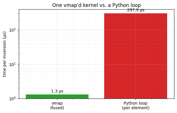

Same solver, but vmap amortises tracing and dispatch across the whole batch — orders of magnitude faster per element than looping, and it composes with jax.jit/grad. For a $d$ -dimensional marginal layer you simply vmap over the leading (batch) axes and apply the scalar solve per coordinate.

Recap¶

Solving $F(x)=u$ :

method	convergence	needs $F'$ ?	robust?	use
bisection	linear ( $2^{-n}$ )	no	always (monotone)	default; `gauss_flows` inverse
Newton	quadratic	yes	no (tails)	when bracketed & well-scaled
safeguarded Newton	quadratic + safe	yes	yes	best of both (Brent-style)

Differentiating the inverse, and scaling it:

technique	gradient	memory	note
unroll bisection	wrong (0)	$O(n)$	comparisons kill the gradient
unroll Newton	correct	$O(n)$	smooth update; memory-heavy
one-step	correct	$O(1)$	detach + 1 Newton step
adjoint	correct	$O(1)$	`optimistix` `ImplicitAdjoint`; automatic
`jax.vmap`	—	—	batch the scalar solve into one kernel

Next up — end of Part 1. We can now build, fit, train, and invert a single 1D marginal transform every way that matters. Part 2 stacks them with rotations (PCA, Householder, random) so that marginal Gaussianization can attack multivariate dependence — the second half of the RBIG loop from Part 0 notebook 04.

References¶

Brent, R. P. (1973). Algorithms for Minimization Without Derivatives. Prentice-Hall.
Kidger, P. (2021). On Neural Differential Equations [Phdthesis]. University of Oxford.
Blondel, M., Berthet, Q., Cuturi, M., Frostig, R., Hoyer, S., Llinares-López, F., Pedregosa, F., & Vert, J.-P. (2022). Efficient and Modular Implicit Differentiation. Advances in Neural Information Processing Systems (NeurIPS).