Mixture-CDF as a learnable bijector

03 — Mixture-CDF as a learnable bijector¶

Notebooks 01–02 fit marginals by quantiles, EM, or plug-in rules. But the whole point of a normalizing flow is that every layer is differentiable in its parameters, so a deep stack can be trained jointly by gradient descent. This notebook treats the mixture-CDF as that learnable layer and trains it end-to-end by maximum likelihood.

What you will see

The flow MLE objective — minimise the negative log-likelihood of the Gaussianized output.
A gauss_flows.MixtureGaussianCDF marginal trained end-to-end with optax (loss curve + learned density), reaching the EM fit by gradient descent so it can train jointly inside a deep flow.

import warnings

warnings.filterwarnings("ignore")

import equinox as eqx
import jax
import jax.numpy as jnp
import jax.scipy.stats as jstats
import matplotlib.pyplot as plt
import numpy as np
import optax

import gauss_flows as gf
from _style import style_ax

jax.config.update("jax_enable_x64", True)
rng = np.random.default_rng(13)

x = jnp.asarray(np.concatenate([rng.normal(-2.0, 0.5, 3000),
                                rng.normal(1.5, 0.8, 3000)])[:, None])

1. The maximum-likelihood objective¶

A marginal bijector $z = T_\theta(x)$ with base $\mathcal{N}(0,1)$ assigns each point the log-density (change of variables, Part 0 notebook 00)

\log p_\theta(x) = \log \phi\big(T_\theta(x)\big) + \log\big|T_\theta'(x)\big|,

((1))

and training maximises the average $\log p_\theta$ — equivalently minimises the negative log-likelihood $\mathcal{L}(\theta) = -\mathbb{E}_x[\log p_\theta(x)]$ . For gauss_flows.MixtureGaussianCDF the parameters θ are the (unconstrained) mixture weights, means, and scales, and both terms above are returned by transform_and_log_det — so $\mathcal{L}$ is a plain differentiable function of θ that optax can descend.

def nll(bijector, xb):
    z, log_det = jax.vmap(bijector.transform_and_log_det)(xb)
    log_px = jnp.sum(jstats.norm.logpdf(z), axis=-1) + log_det
    return -jnp.mean(log_px)


# Start from a deliberately rough init, then learn the parameters end-to-end.
init = gf.MixtureGaussianCDF.from_data(x[::20], n_components=6)  # under-fit warm start
params, static = eqx.partition(init, eqx.is_inexact_array)
opt = optax.adam(1e-2)
opt_state = opt.init(params)


@eqx.filter_jit
def train_step(params, opt_state):
    loss, grads = eqx.filter_value_and_grad(
        lambda p: nll(eqx.combine(p, static), x))(params)
    updates, opt_state = opt.update(grads, opt_state)
    return eqx.apply_updates(params, updates), opt_state, loss


losses = []
for _ in range(200):
    params, opt_state, loss = train_step(params, opt_state)
    losses.append(float(loss))

trained = eqx.combine(params, static)
print(f"NLL: {losses[0]:.4f} (init) -> {losses[-1]:.4f} (trained)")

NLL: 1.7441 (init) -> 1.6490 (trained)

grid = jnp.linspace(-5, 5, 400)[:, None]
# density of the trained marginal: p(x) = phi(T(x)) * |T'(x)| = exp(logphi + logdet)
zt, ldt = jax.vmap(trained.transform_and_log_det)(grid)
dens_trained = np.exp(np.asarray(jstats.norm.logpdf(zt).sum(-1) + ldt))

fig, axes = plt.subplots(1, 2, figsize=(11, 4.2))
axes[0].plot(losses, color="tab:purple", lw=1.8)
axes[0].set(title="end-to-end MLE training", xlabel="Adam step",
            ylabel="negative log-likelihood")
style_ax(axes[0])

axes[1].hist(np.asarray(x)[:, 0], bins=60, density=True, color="tab:blue", alpha=0.5,
             label="data")
axes[1].plot(np.asarray(grid).ravel(), dens_trained, color="tab:red", lw=2,
             label="trained mixture-CDF density")
axes[1].set(title="learned marginal density", xlabel="x", ylabel="density")
axes[1].legend(fontsize=8); style_ax(axes[1])
fig.tight_layout()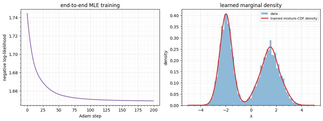

The NLL falls and the learned density (red) locks onto the bimodal data — the same fit EM gave in notebook 01, but reached by gradient descent. That difference is the whole point: because the layer is differentiable in θ, it drops into a deep flow and trains jointly with every rotation and coupling around it, instead of being fit in isolation.

Training used only the forward gradient (jax.grad of transform_and_log_det, all closed-form). The moment you instead train through the layer’s inverse — e.g. a sampling- or variational objective — you hit the root-find gradient question, which notebook 04 answers.

Recap¶

piece	takeaway	in code
log-density	$\log\phi(T_\theta x) + \log\lvert T_\theta'\rvert$	`transform_and_log_det`
MLE objective	minimise NLL of the Gaussianized output	`nll`
end-to-end training	gradient descent in θ; stacks into deep flows	`optax` + `eqx.filter_value_and_grad`
forward gradient	closed form — all MLE needs	plain `jax.grad`
inverse gradient	unroll / one-step / adjoint	notebook 04

Next up. Training leaned on the closed-form forward map. The inverse is a root-find, and 04 — Inversion strategies covers it end to end: bisection vs. Newton, the safeguarded hybrid, how to differentiate the inverse (and why unrolling can fail), and how to vectorise it across a batch.