KDE & Gaussian-mixture CDFs

01 — KDE & Gaussian-mixture CDFs¶

The empirical CDF of notebook 00 is consistent but jagged (a staircase, not differentiable) and tail-blind (nothing beyond the data). Both problems vanish if we estimate a smooth density and integrate it into a CDF. Two estimators dominate practice: a kernel density estimate (nonparametric) and a Gaussian mixture (parametric) — the latter is the marginal bijector at the heart of gauss_flows.

What you will see

A KDE-based CDF Gaussianization (rbig.KDEGaussianizer) — smooth where the ECDF was a staircase.
The Gaussian-mixture CDF $F(x)=\sum_k\pi_k\Phi(\tfrac{x-\mu_k}{\sigma_k})$ : closed-form forward, differentiable, invertible by root-find — the workhorse gauss_flows.MixtureGaussianCDF.
Choosing the bandwidth $h$ (KDE) and the component count $K$ (mixture, via BIC) — the bias/variance knob of each.

import warnings

warnings.filterwarnings("ignore")

import jax
import jax.numpy as jnp
import matplotlib.pyplot as plt
import numpy as np
from scipy import stats
from sklearn.mixture import GaussianMixture

import gauss_flows as gf
import rbig
from _style import GAUSS_KW, style_ax

jax.config.update("jax_enable_x64", True)
rng = np.random.default_rng(11)

# A clearly bimodal marginal so the bandwidth / component count matter visibly.
x = np.concatenate([rng.normal(-2.0, 0.5, 3000),
                    rng.normal(1.5, 0.8, 3000)])[:, None]
grid = np.linspace(-5, 5, 500)

1. KDE-based CDF¶

A kernel density estimate sums a smooth bump at each sample,

\hat f_h(x) = \frac{1}{nh}\sum_{i=1}^n K\!\Big(\frac{x-x_i}{h}\Big), \qquad \hat F_h(x) = \int_{-\infty}^{x}\hat f_h\,,

((1))

and with a Gaussian kernel that integral is itself a sum of normal CDFs — so $\hat F_h$ is smooth and strictly increasing, exactly what the probability integral transform wants. rbig.KDEGaussianizer builds $\Phi^{-1}(\hat F_h(x))$ .

kde = rbig.KDEGaussianizer().fit(x)
z_kde = kde.transform(x)


def ecdf(s, t):
    return np.searchsorted(np.sort(s), t, side="right") / len(s)


fig, axes = plt.subplots(1, 2, figsize=(11, 4.2))
axes[0].hist(x[:, 0], bins=60, density=True, color="tab:blue", alpha=0.5, label="data")
axes[0].plot(grid, stats.gaussian_kde(x[:, 0])(grid), color="tab:red", lw=2,
             label="KDE density $\\hat f_h$")
axes[0].set(title="KDE smooths the histogram", xlabel="x", ylabel="density")
axes[0].legend(fontsize=8); style_ax(axes[0])

axes[1].step(grid, ecdf(x[:, 0], grid), where="post", color="tab:gray", lw=1.2,
             label="ECDF (staircase)")
axes[1].plot(grid, stats.gaussian_kde(x[:, 0]).integrate_box_1d(-np.inf, grid[0])
             + np.cumsum(stats.gaussian_kde(x[:, 0])(grid)) * (grid[1] - grid[0]),
             color="tab:red", lw=2, label="KDE CDF $\\hat F_h$ (smooth)")
axes[1].set(title="...and gives a smooth, invertible CDF", xlabel="x", ylabel="F(x)")
axes[1].legend(fontsize=8); style_ax(axes[1])
fig.tight_layout()

print(f"KDE Gaussianize: output std = {z_kde.std():.3f}, "
      f"round-trip err = {np.abs(x - kde.inverse_transform(z_kde)).max():.2e}")

KDE Gaussianize: output std = 0.940, round-trip err = 4.99e-13

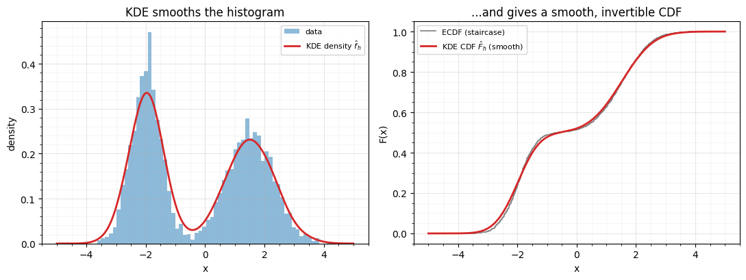
The red KDE density traces both modes, and its CDF is the smooth curve the ECDF staircase was approximating. The Gaussianized output is unit-variance and round-trips cleanly — no tail blow-up, because the kernel tails extend past the data automatically.

2. The Gaussian-mixture CDF¶

The parametric workhorse fits a mixture of $K$ Gaussians and uses its CDF directly,

F(x) = \sum_{k=1}^{K}\pi_k\,\Phi\!\Big(\frac{x-\mu_k}{\sigma_k}\Big), \qquad z = \Phi^{-1}\big(F(x)\big).

((2))

The forward map is a closed-form, differentiable sum; the inverse is the monotone root-find of Part 0 notebook 02; and the log-det is $\log f(x) - \log\phi(z)$ . This is rbig.GMMGaussianizer and gauss_flows.MixtureGaussianCDF — the marginal layer every parametric Gaussianization flow stacks.

b = gf.MixtureGaussianCDF.from_data(jnp.asarray(x), n_components=2)
z_mix, logdet = jax.vmap(b.transform_and_log_det)(jnp.asarray(x))
x_rt = jax.vmap(b.inverse)(z_mix)

gm = GaussianMixture(2, random_state=0).fit(x)
dens = np.exp(gm.score_samples(grid[:, None]))
cdf = np.array([np.sum(gm.weights_ * stats.norm.cdf(t, gm.means_.ravel(),
                np.sqrt(gm.covariances_.ravel()))) for t in grid])

fig, axes = plt.subplots(1, 3, figsize=(12, 3.6))
axes[0].hist(x[:, 0], bins=60, density=True, color="tab:blue", alpha=0.5)
axes[0].plot(grid, dens, color="tab:red", lw=2, label="2-component mixture")
axes[0].set(title="fitted mixture density", xlabel="x"); axes[0].legend(fontsize=8)
axes[1].plot(grid, cdf, color="tab:red", lw=2)
axes[1].set(title=r"mixture CDF $F(x)=\sum_k\pi_k\Phi$", xlabel="x", ylabel="F(x)")
zz = np.linspace(-4, 4, 200)
axes[2].hist(np.asarray(z_mix)[:, 0], bins=50, density=True, color="tab:green", alpha=0.6)
axes[2].plot(zz, stats.norm.pdf(zz), **GAUSS_KW, label=r"$\mathcal{N}(0,1)$")
axes[2].set(title=r"$z=\Phi^{-1}(F(x))$", xlabel="z"); axes[2].legend(fontsize=8)
for a in axes:
    style_ax(a)
fig.tight_layout()

print(f"MixtureGaussianCDF: output std = {float(z_mix.std()):.3f}, "
      f"round-trip err = {float(jnp.max(jnp.abs(jnp.asarray(x) - x_rt))):.2e}, "
      f"log-det finite = {bool(jnp.all(jnp.isfinite(logdet)))}")

MixtureGaussianCDF: output std = 0.863, round-trip err = 8.93e-14, log-det finite = True

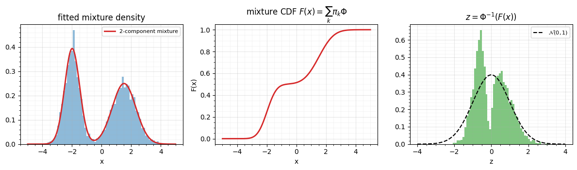
The two-component mixture nails the bimodal density, its CDF is smooth and monotone, and the Gaussianized output is a clean standard normal — round-tripping to ~10^-14 (the tail-inverse fix from gauss_flows#108). Unlike the KDE, the mixture has only $3K$ parameters, is trivially differentiable in them, and extrapolates sensibly — which is why it is the parametric default.

3. Choosing the knob: bandwidth $h$ and components $K$ ¶

Each estimator has one capacity knob, and it is the usual bias/variance trade-off.

KDE bandwidth $h$ . Too small and $\hat f_h$ is a spiky over-fit (high variance); too large and it smears the two modes into one (high bias). Plug-in rules like Scott’s / Silverman’s Silverman (1986) give a sane default.

fig, axes = plt.subplots(1, 2, figsize=(11, 4.2))
for bw, label, c in [(0.05, "h too small (spiky)", "tab:orange"),
                     ("scott", "Scott's rule (good)", "tab:green"),
                     (0.6, "h too large (oversmoothed)", "tab:red")]:
    axes[0].plot(grid, stats.gaussian_kde(x[:, 0], bw_method=bw)(grid), lw=1.8,
                 label=label, color=c)
axes[0].hist(x[:, 0], bins=60, density=True, color="tab:blue", alpha=0.3)
axes[0].set(title="KDE bandwidth: bias vs. variance", xlabel="x", ylabel="density")
axes[0].legend(fontsize=8); style_ax(axes[0])

# Mixture: BIC selects K (penalised likelihood) on a held-out split.
Ks = np.arange(1, 8)
bic = [GaussianMixture(k, random_state=0).fit(x).bic(x) for k in Ks]
axes[1].plot(Ks, bic, "-o", color="tab:purple", ms=5)
axes[1].plot(Ks[np.argmin(bic)], min(bic), "k*", ms=16,
             label=f"BIC min at K={Ks[np.argmin(bic)]}")
axes[1].set(title="Mixture component count: BIC", xlabel="K (components)", ylabel="BIC")
axes[1].legend(fontsize=8); style_ax(axes[1])
fig.tight_layout()

print("BIC by K:", {int(k): round(v) for k, v in zip(Ks, bic)})

BIC by K: {1: 24593, 2: 19821, 3: 19873, 4: 19906, 5: 19939, 6: 19961, 7: 19984}

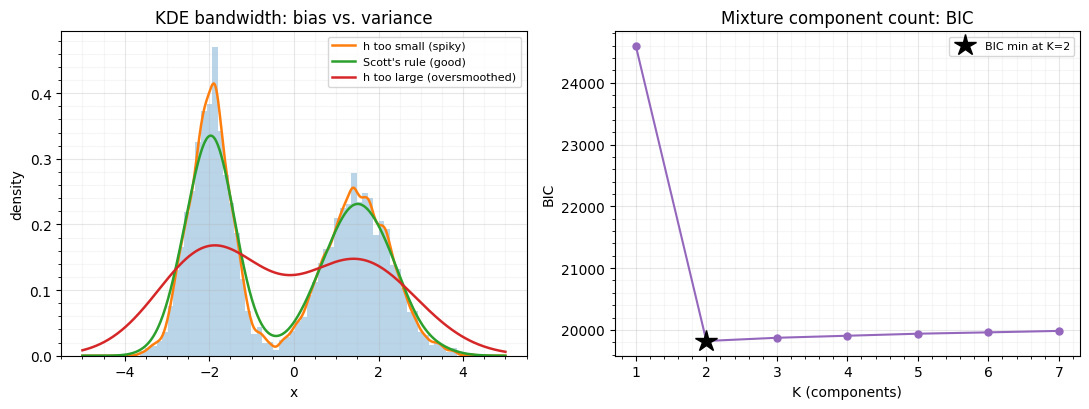
Left: the bandwidth sweep — the spiky orange curve would inject phantom wiggles into the CDF (and noisy gradients), while the oversmoothed red one erases the valley between modes. Right: BIC (log-likelihood penalised by parameter count) bottoms out at $K=2$ , the true number of modes — adding components past that buys no likelihood worth the penalty. Cross-validated held-out likelihood tells the same story.

4. The Jacobian — a smooth log-determinant¶

To use a marginal in a flow we need its per-coordinate log-determinant, the gradient $T'(x)=\mathrm{d}z/\mathrm{d}x$ of $z=\Phi^{-1}(F(x))$ :

\frac{\mathrm{d}z}{\mathrm{d}x} = \frac{f(x)}{\varphi(z)}, \qquad \log\big|T'(x)\big| = \log f(x) - \log\varphi(z), \qquad f(x) = \sum_k \pi_k\,\mathcal{N}(x;\mu_k,\sigma_k).

((3))

Unlike the histogram’s piecewise-constant $f$ (notebook 00), the mixture density is smooth, so the log-det is smooth and differentiable — what gradient training needs. gauss_flows.MixtureGaussianCDF.transform_and_log_det returns exactly this $\log|T'|$ ; we confirm it against an autodiff Jacobian.

bj = gf.MixtureGaussianCDF.from_data(jnp.asarray(x), n_components=2)
xj = jnp.linspace(-5, 5, 600)[:, None]
zj, logdet = jax.vmap(bj.transform_and_log_det)(xj)
dzdx_auto = jax.vmap(lambda v: jax.jacfwd(bj.transform)(v).reshape(()))(xj)
f_mix = np.exp(np.asarray(logdet)) * stats.norm.pdf(np.asarray(zj).ravel())  # f = |T'|*phi(z)

print("log|T'| from transform_and_log_det vs autodiff: max|Δ| = "
      f"{float(jnp.max(jnp.abs(logdet - jnp.log(jnp.abs(dzdx_auto))))):.2e}")

fig, axes = plt.subplots(1, 2, figsize=(11, 4.2))
axes[0].plot(np.asarray(xj).ravel(), f_mix, color="tab:red", lw=2)
axes[0].set(title=r"mixture density $f(x)$ (smooth)", xlabel="x", ylabel="$f(x)$")
style_ax(axes[0])
axes[1].plot(np.asarray(xj).ravel(), np.asarray(logdet), color="tab:purple", lw=2)
axes[1].set(title=r"log-determinant $\log|T'(x)| = \log f(x) - \log\varphi(z)$",
            xlabel="x", ylabel=r"$\log|T'(x)|$")
style_ax(axes[1])
fig.tight_layout()

log|T'| from transform_and_log_det vs autodiff: max|Δ| = 3.23e-15

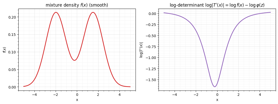
The package log-det matches autodiff to machine precision, and both are smooth functions of $x$ — the low-density valley between the two modes is the central dip in $\log|T'|$ , which then rises toward the tails as $\varphi(z)\to 0$ . This smooth, exact log-det is precisely the per-coordinate term a flow sums in log_prob.

Recap¶

estimator	CDF	knob	selector
KDE	sum of kernel CDFs (smooth)	bandwidth $h$	Scott/Silverman, CV
Gaussian mixture	$\sum_k\pi_k\Phi$ (closed form)	components $K$	BIC / held-out NLL

tool	role
`rbig.KDEGaussianizer`	nonparametric smooth marginal
`rbig.GMMGaussianizer` / `gf.MixtureGaussianCDF`	parametric marginal bijector

Next up. Mixtures are smooth and compact but their inverse needs a root-find. 02 — Monotone-spline CDFs builds marginals from monotone splines — including the rational-quadratic spline with an exact analytic inverse, the bijector behind modern neural spline flows.

References¶

Silverman, B. W. (1986). Density Estimation for Statistics and Data Analysis. Chapman.