Block-tridiagonal operators — precision form for Markov / state-space GPs
A block-tridiagonal matrix has non-zero blocks only on its main diagonal and the two adjacent diagonals; everywhere else is zero. This is the precision form of any Markov chain — Kalman filters, hidden Markov models, AR processes, discretized linear SDEs all live here. Storage is instead of , and every primitive (cholesky, solve, logdet, diag) drops from to via a banded forward-backward sweep.
This is the temporal-Markov dual of Toeplitz: where Toeplitz exploits stationarity (constant diagonals, dense in covariance form), block-tridiagonal exploits conditional independence (banded sparsity in precision form). Many state-space GP workflows convert from one to the other deliberately — covariance form is dense but stationary, precision form is sparse but Markov, and the right choice depends on which primitive dominates your cost.
0. Where block-tridiagonal precision shows up in geoscience
A non-exhaustive list — every one of these is an operator-typed BlockTriDiag in gaussx:
- Kalman filtering / smoothing on geophysical timeseries: trajectory estimation for GPS displacements, sea-level reconstruction, gravimeter records, magnetometer drift correction. The full smoothed posterior precision over all time-steps is exactly block-tridiagonal — the Markov property means past and future are conditionally independent given the present, which forces the precision into this banded form.
- State-space GP regression: every Matérn kernel of half-integer order has a finite-dimensional state-space representation; on a regular time grid the resulting joint precision is block-tridiagonal with block size = state dimension (1 for Matérn-1/2, 2 for 3/2, 3 for 5/2). Hartikainen & Särkkä (2010) gave the systematic recipe; this is what makes Matérn GPs scale to billions of points in temporal seismology, climate reconstructions, and remote-sensing time series.
- Discretized linear SDEs / OU processes: the Ornstein–Uhlenbeck precision on a regular grid is exactly block-tridiagonal with blocks — the diagonal is , the sub-diagonal is .
- 1-D GMRF priors for inverse problems: the second-difference precision on a regular grid (encoding a smoothness prior for inversions, e.g. seismic-velocity profiles or ice-thickness estimation) is tridiagonal with blocks of size 1.
- Spacetime separable models: when one axis is Markov and the other is general (e.g. Markov in time × dense in space), the precision factorizes as
Kronecker(BlockTriDiag, K_space)— used heavily in animal-movement modelling, ENSO state-space filters, and ocean-data assimilation. - Filtering with non-Gaussian likelihoods (Newton / Laplace approximations): each Newton step against a state-space prior produces a block-tridiagonal posterior precision (prior + diagonal Hessian sites = block-tridiagonal sum). Used in extended Kalman smoothing, log-Gaussian Cox processes for earthquake catalogs, Bayesian filtering of gridded environmental observations.
The mental shortcut: if your process is Markov in one of its dimensions, the precision is block-tridiagonal in that dimension. Banded sparsity is the language of conditional independence.
from __future__ import annotations

import warnings
warnings.filterwarnings("ignore", message=r".*IProgress.*")

import einx
import jax
import jax.numpy as jnp
import lineax as lx
import matplotlib.pyplot as plt
import numpy as np
from gaussx import (
    BlockTriDiag,
    LowerBlockTriDiag,
    cholesky,
    logdet,
    solve,
)

jax.config.update("jax_enable_x64", True)
KEY = jax.random.PRNGKey(0)
plt.rcParams.update({
    "figure.dpi": 110,
    "axes.grid": True,
    "axes.grid.which": "both",
    "xtick.minor.visible": True,
    "ytick.minor.visible": True,
    "grid.alpha": 0.3,
})
1. The block-tridiagonal precision
A symmetric block-tridiagonal precision matrix is parameterized by diagonal blocks and sub-diagonal blocks :
Storage: blocks of size on the diagonal plus off-diagonal blocks. Total: floats — linear in instead of quadratic.
The shape encodes the Markov assumption: whenever in block coordinates means for non-adjacent blocks — past and future are conditionally independent given the present.
# A small AR(1)-like precision with d=2 latent state per timestep
N, d = 6, 2
phi, sigma2 = 0.7, 1.0

# Identity-block AR(1) precision: D_k = (1 + ϕ²)/σ² · I,  A_k = -ϕ/σ² · I
D_blocks = jnp.tile(((1.0 + phi**2) / sigma2) * jnp.eye(d), (N, 1, 1))
A_blocks = jnp.tile((-phi / sigma2) * jnp.eye(d), (N - 1, 1, 1))
# Boundary: marginal-stationary endpoints
D_blocks = D_blocks.at[0].set((1.0 / sigma2) * jnp.eye(d))
D_blocks = D_blocks.at[-1].set((1.0 / sigma2) * jnp.eye(d))

Lam = BlockTriDiag(D_blocks, A_blocks, tags=lx.positive_semidefinite_tag)

# Visualize the sparsity pattern
fig, ax = plt.subplots(figsize=(5.5, 5.5))
M = Lam.as_matrix()
ax.imshow(jnp.where(jnp.abs(M) > 1e-12, jnp.abs(M), jnp.nan),
          cmap="viridis", aspect="equal")
for k in range(1, N):
    ax.axhline(k * d - 0.5, color="white", lw=0.5)
    ax.axvline(k * d - 0.5, color="white", lw=0.5)
ax.set_title(rf"Block-tridiagonal precision $\Lambda$  (N={N}, d={d})")
ax.set_xlabel("col"); ax.set_ylabel("row")
plt.tight_layout()
plt.show()

print(f"size           : {Lam._size} x {Lam._size}")
print(f"storage (BTD)  : {(2*N - 1) * d * d} floats")
print(f"storage (dense): {Lam._size**2} floats   ({Lam._size**2 / ((2*N - 1)*d*d):.0f}x more)")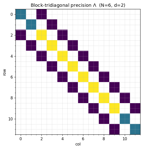
size           : 12 x 12
storage (BTD)  : 44 floats
storage (dense): 144 floats   (3x more)
2. Banded matvec & Cholesky in 
The matvec sweeps once through the blocks:
— three block-matvecs per row, total .
The Cholesky factor of a symmetric positive-definite block-tridiagonal matrix is lower block-bidiagonal — same banded shape, just lower-triangular. gaussx.cholesky(BlockTriDiag) returns a LowerBlockTriDiag and runs the banded Cholesky sweep in flops:
This is exactly the Kalman filter forward sweep written in matrix language. Once is in hand, every downstream primitive (solve, logdet, sampling) is one or two banded back-substitutions, also .
# Verify matvec
v = jax.random.normal(jax.random.PRNGKey(1), (N * d,))
ref = M @ v
print(f"matvec error : {jnp.linalg.norm(Lam.mv(v) - ref):.2e}")

# Cholesky lands in the banded factor type
L_op = cholesky(Lam)
print(f"\ncholesky type    : {type(L_op).__name__}")
print(f"factor matches L : {jnp.allclose(L_op.as_matrix() @ L_op.as_matrix().T, M, atol=1e-10)}")

# Solve via banded forward-backward sweep
b = jnp.ones(N * d)
x_struct = solve(Lam, b)
x_dense  = jnp.linalg.solve(M, b)
print(f"solve error      : {jnp.linalg.norm(x_struct - x_dense):.2e}")

# logdet via 2 sum log diag(L)
ld_struct = float(logdet(Lam))
ld_dense  = float(jnp.linalg.slogdet(M)[1])
print(f"logdet (struct)  : {ld_struct:.6f}")
print(f"logdet (dense)   : {ld_dense:.6f}")
matvec error : 1.11e-16
cholesky type    : LowerBlockTriDiag
factor matches L : True
solve error : 1.26e-15
logdet (struct)  : -1.346689
logdet (dense)   : -1.346689
3. Cost table — banded vs dense
With blocks of size (total dimension ):
| Operation | Dense | BlockTriDiag |
|---|---|---|
| Storage | ||
| Matvec | ||
| Cholesky | ||
| Solve (after Cholesky) | ||
| logdet | ||
| Sample |
Linear in across the board — the asymptotic gap from to is what makes million-step state-space GP regression tractable. For Matérn-3/2 in time, and can be 107 on a single GPU; the dense form is unimaginable at that scale.
# Theoretical FLOP plot: dense vs banded Cholesky as N grows
Ns = np.array([2**k for k in range(4, 18)])  # 16 .. 130k
d = 2
dense_chol  = (1/3) * (Ns * d)**3
banded_chol = Ns * d**3
dense_mv    = 2 * (Ns * d)**2
banded_mv   = 5 * Ns * d**2

fig, ax = plt.subplots(figsize=(7.5, 5.5))
ax.loglog(Ns, dense_chol,  "C3-",  marker="o", label=r"dense Cholesky $O(N^3 d^3)$")
ax.loglog(Ns, banded_chol, "C2-",  marker="s", label=r"banded Cholesky $O(N d^3)$")
ax.loglog(Ns, dense_mv,    "C3--", marker="o", label=r"dense matvec $O(N^2 d^2)$")
ax.loglog(Ns, banded_mv,   "C2--", marker="s", label=r"banded matvec $O(N d^2)$")
ax.set_xlabel(r"number of blocks $N$  ($d=2$)")
ax.set_ylabel("FLOPs (theoretical)")
ax.set_title("Block-tridiagonal vs dense — Cholesky and matvec scaling")
ax.legend(loc="upper left")
plt.tight_layout()
plt.show()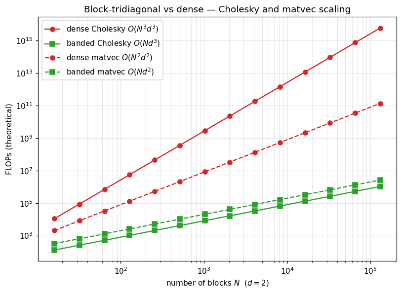
4. Sampling and conditional smoothing
Drawing from a precision-form Gaussian uses the Cholesky factor via with — a backward triangular solve through the banded factor, total.
In Kalman-smoother language:
- Forward sweep = Cholesky of Λ (the prediction + update steps).
- Backward sweep = solve (the RTS / two-filter smoothing pass).
The two sweeps over the banded factor are the smoothing algorithm written in matrix-vector primitives. Everything that’s commonly written as filter recursions is already there in solve(BlockTriDiag, …).
# Build a longer chain and sample from N(0, Λ⁻¹) using the banded Cholesky
N_long, d = 200, 1
phi, sigma2 = 0.92, 1.0
D_long = jnp.tile(((1.0 + phi**2) / sigma2) * jnp.eye(d), (N_long, 1, 1))
A_long = jnp.tile((-phi / sigma2) * jnp.eye(d), (N_long - 1, 1, 1))
D_long = D_long.at[0].set((1.0 / sigma2) * jnp.eye(d))
D_long = D_long.at[-1].set((1.0 / sigma2) * jnp.eye(d))
Lam_long = BlockTriDiag(D_long, A_long, tags=lx.positive_semidefinite_tag)
L_long = cholesky(Lam_long)

# Sample by solving L^T x = z  (precision-form sampling)
keys = jax.random.split(jax.random.PRNGKey(2), 5)
samples = []
for k in keys:
    z = jax.random.normal(k, (N_long * d,))
    # x = L^{-T} z  via a triangular solve on the lower-bidiagonal factor
    x = jax.scipy.linalg.solve_triangular(L_long.as_matrix().T, z, lower=False)
    samples.append(np.asarray(x).flatten())

fig, ax = plt.subplots(figsize=(8, 4))
for i, s in enumerate(samples):
    ax.plot(s, alpha=0.7, label=f"sample {i+1}")
ax.set_xlabel("time index")
ax.set_ylabel("$x_t$")
ax.set_title(rf"Five samples from AR(1) with $\phi$={phi}, parameterized as block-tridiagonal precision (N={N_long})")
ax.legend(loc="upper right", fontsize=8, ncol=5)
plt.tight_layout()
plt.show()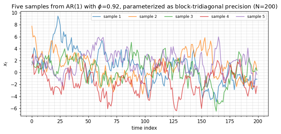
5. Prior + diagonal likelihood = block-tridiagonal posterior
The shape is closed under adding diagonal precision (Gaussian likelihood / Newton sites). If is block-tridiagonal and is block-diagonal (one Hessian block per timestep, e.g. from a Gaussian observation model), then
is also block-tridiagonal — gaussx.BlockTriDiag exposes __add__ / __sub__ / __mul__ so you can write this directly without leaving the structured class. This is exactly the Newton step against a state-space prior that powers extended-Kalman smoothing, IPP filtering for Cox processes, and the Bayesian-filtering literature for non-conjugate observation models.
# Posterior precision = prior + diagonal likelihood
# Likelihood: Gaussian observations with per-timestep precision w_k
W_blocks = jnp.tile(2.0 * jnp.eye(d), (N_long, 1, 1))   # 1/σ²_obs = 2.0
A_zero = jnp.zeros_like(A_long)
W_op = BlockTriDiag(W_blocks, A_zero)

Lam_post = Lam_long + W_op
print(f"posterior type     : {type(Lam_post).__name__}")
print(f"posterior is BTD   : {isinstance(Lam_post, BlockTriDiag)}")
print(f"posterior shape    : {Lam_post._size}")

# The added structure is preserved — same banded primitives still apply.
ld_post = float(logdet(BlockTriDiag(Lam_post.diagonal, Lam_post.sub_diagonal,
                                    tags=lx.positive_semidefinite_tag)))
print(f"posterior logdet   : {ld_post:.4f}")
posterior type : BlockTriDiag
posterior is BTD : True
posterior shape : 200
posterior logdet : 256.3895
6. The covariance ↔ precision duality
Two ways to encode the same Markov GP:
| Form | Storage | Dense in | Sparse in | Cheap primitive |
|---|---|---|---|---|
| Covariance | dense (Toeplitz if stationary) | covariance | nothing | matvec via FFT (Toeplitz) |
| Precision | block-tridiagonal | precision | $ | i-j |
Choose by what the workload needs:
- Filtering / smoothing / sampling / likelihood evaluation → precision form,
BlockTriDiag. - Pure prediction at new timepoints from a stationary kernel → covariance form,
Toeplitz. - Both → keep both; convert as needed.
gaussx’s state-space primitives handle the conversion when you need it.
The next notebook (1.6 MaskedOperator) covers the missing-data variant of this story: when observations are sampled at a subset of grid points, you wrap a Toeplitz or BlockTriDiag operator in a mask that picks out the observed indices, preserving structure on the prior side while correctly accounting for the holes in the data.