Kronecker Eigendecomposition - Research Notebook

For a Kronecker product $A \otimes B$ , all eigenvalues and eigenvectors decompose per-factor:

\lambda_{ij} = \lambda_i^A \cdot \lambda_j^B, \qquad v_{ij} = v_i^A \otimes v_j^B

((1))

This means we can compute the full spectrum of an $N \times N$ matrix ( $N = n_1 n_2$ ) by only decomposing two small matrices. gaussx exploits this for cholesky, sqrt, logdet, and inv.

Context¶

The Kronecker eigendecomposition is a special case of the tensor product spectral theorem. If $A = U_A \Lambda_A U_A^\top$ and $B = U_B \Lambda_B U_B^\top$ , then

A \otimes B = (U_A \otimes U_B)\,(\Lambda_A \otimes \Lambda_B)\,(U_A \otimes U_B)^\top.

((2))

This result is foundational for:

GP inference on grids -- computing solves and log-determinants without forming the full $N \times N$ matrix (Saatci, 2012).
Solving Kronecker-structured linear systems -- reducing an $N$ -dimensional problem to two smaller per-factor problems.
Stochastic PDEs with separable operators -- exploiting product structure in spatial and temporal discretizations.

from __future__ import annotations

import warnings


warnings.filterwarnings("ignore", message=r".*IProgress.*")

import jax
import jax.numpy as jnp
import lineax as lx
import matplotlib.pyplot as plt

import gaussx


jax.config.update("jax_enable_x64", True)

Setup: PSD Kronecker product¶

key = jax.random.PRNGKey(42)
k1, k2 = jax.random.split(key)

n1, n2 = 8, 10
N = n1 * n2

# Random PSD matrices
M1 = jax.random.normal(k1, (n1, n1))
A = M1 @ M1.T + 0.1 * jnp.eye(n1)

M2 = jax.random.normal(k2, (n2, n2))
B = M2 @ M2.T + 0.1 * jnp.eye(n2)

A_op = lx.MatrixLinearOperator(A, lx.positive_semidefinite_tag)
B_op = lx.MatrixLinearOperator(B, lx.positive_semidefinite_tag)
K = gaussx.Kronecker(A_op, B_op)

print(f"A: {n1}x{n1}, B: {n2}x{n2}")
print(f"A kron B: {N}x{N} = {N**2:,} entries")

A: 8x8, B: 10x10
A kron B: 80x80 = 6,400 entries

Per-factor eigenvalues¶

eigs_A = jnp.linalg.eigvalsh(A)
eigs_B = jnp.linalg.eigvalsh(B)

# Kronecker eigenvalues = outer product of per-factor eigenvalues
eigs_kron = jnp.sort(jnp.outer(eigs_A, eigs_B).ravel())

# Dense eigenvalues (for verification)
eigs_dense = jnp.linalg.eigvalsh(K.as_matrix())

print(f"Per-factor eigenvalues: {n1} + {n2} = {n1 + n2} eigh calls")
print(f"Dense eigenvalues: one {N}x{N} eigh call")
print(f"Max eigenvalue error: {jnp.max(jnp.abs(eigs_kron - eigs_dense)):.2e}")

Per-factor eigenvalues: 8 + 10 = 18 eigh calls
Dense eigenvalues: one 80x80 eigh call

Max eigenvalue error: 2.84e-13

fig, axes = plt.subplots(1, 3, figsize=(14, 3.5))

axes[0].stem(range(n1), eigs_A, linefmt="C0-", markerfmt="C0o", basefmt="k-")
axes[0].set_title(f"Eigenvalues of A ({n1}x{n1})")
axes[0].set_xlabel("Index")
axes[0].set_ylabel("$\\lambda$")
axes[0].grid(True, which="major", alpha=0.3)
axes[0].grid(True, which="minor", alpha=0.1)
axes[0].minorticks_on()

axes[1].stem(range(n2), eigs_B, linefmt="C1-", markerfmt="C1o", basefmt="k-")
axes[1].set_title(f"Eigenvalues of B ({n2}x{n2})")
axes[1].set_xlabel("Index")
axes[1].grid(True, which="major", alpha=0.3)
axes[1].grid(True, which="minor", alpha=0.1)
axes[1].minorticks_on()

axes[2].semilogy(eigs_kron, "C2-", lw=2, label="Kronecker (per-factor)")
axes[2].semilogy(eigs_dense, "k--", lw=1.5, label="Dense (verification)")
axes[2].set_title(f"Eigenvalues of A$\\otimes$B ({N}x{N})")
axes[2].set_xlabel("Index")
axes[2].legend(fontsize=9)
axes[2].grid(True, which="major", alpha=0.3)
axes[2].grid(True, which="minor", alpha=0.1)
axes[2].minorticks_on()

plt.tight_layout()
plt.show()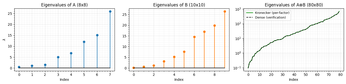

Structured Cholesky¶

cholesky(A kron B) = cholesky(A) kron cholesky(B)

L = gaussx.cholesky(K)
print(f"cholesky type: {type(L).__name__}")

# Reconstruction error
recon = L.as_matrix() @ L.as_matrix().T
print(f"||L L^T - K||_max: {jnp.max(jnp.abs(recon - K.as_matrix())):.2e}")

cholesky type: Kronecker

||L L^T - K||_max: 5.68e-14

Structured sqrt¶

sqrt(A kron B) = sqrt(A) kron sqrt(B)

S = gaussx.sqrt(K)
print(f"sqrt type: {type(S).__name__}")

# Verify S @ S = K
recon_sqrt = S.as_matrix() @ S.as_matrix()
print(f"||S S - K||_max: {jnp.max(jnp.abs(recon_sqrt - K.as_matrix())):.2e}")

sqrt type: Kronecker
||S S - K||_max: 4.41e-13

Structured logdet¶

$\log|A \otimes B| = n_2 \log|A| + n_1 \log|B|$

Derivation. Using the Kronecker eigenvalues $\lambda_{ij} = \lambda_i^A \lambda_j^B$ :

\log|A \otimes B| = \sum_{i,j} \log(\lambda_i^A \, \lambda_j^B) = \sum_{i,j} \bigl(\log \lambda_i^A + \log \lambda_j^B\bigr) = n_2 \sum_i \log \lambda_i^A + n_1 \sum_j \log \lambda_j^B = n_2 \log|A| + n_1 \log|B|.

((3))

ld_structured = gaussx.logdet(K)
ld_dense = jnp.linalg.slogdet(K.as_matrix())[1]
ld_from_eigs = jnp.sum(jnp.log(eigs_kron))

print(f"Structured logdet:  {ld_structured:.6f}")
print(f"Dense logdet:       {ld_dense:.6f}")
print(f"From eigenvalues:   {ld_from_eigs:.6f}")

Structured logdet:  233.876851
Dense logdet:       233.876851
From eigenvalues:   233.876851

Summary¶

Operation	Dense cost	Kronecker cost	Speedup
Eigenvalues	O(N^3)	O(n1^3 + n2^3)	~N/n_max
Cholesky	O(N^3)	O(n1^3 + n2^3)	~N/n_max
Logdet	O(N^3)	O(n1^3 + n2^3)	~N/n_max
Solve	O(N^3)	O(n1^3 + n2^3)	~N/n_max

References¶

Van Loan, C. F. (2000). The ubiquitous Kronecker product. Journal of Computational and Applied Mathematics, 123, 85--100.
Saatci, Y. (2012). Scalable Inference for Structured Gaussian Process Models. PhD thesis, University of Cambridge.
Steeb, W.-H. (2011). Matrix Calculus and Kronecker Product. 2nd edition, World Scientific.