KroneckerSum vs SumKronecker — two operators, one confusing name

Two of the most useful structured operators in gaussx have nearly identical names — and very different jobs. Sorting them out is worth a notebook of its own.

Operator	Definition	Where it appears
`KroneckerSum` $A\oplus B$	$A\otimes I_b + I_a\otimes B$	separable PDEs, spacetime GMRF priors, additive Gaussian fields
`SumKronecker`	$A_1\otimes B_1 + A_2\otimes B_2$	multi-output GPs with correlated tasks, signal + iid noise on a grid

Both produce $n_a n_b \times n_a n_b$ matrices. Both look like “a sum of Kroneckers”. But the structure is wildly different: KroneckerSum is the additive separation of two operators acting on independent axes — eigendecomposable in closed form via the eigendecomposition of each factor alone. SumKronecker is the superposition of two unrelated Kronecker products — generally not jointly diagonalizable, and requiring an $O((n_a n_b)^3)$ inner solve.

What you will see by the end:

The vec-form identity that makes KroneckerSum matvec cost $O(n_a n_b(n_a + n_b))$ .
The eigendecomposition $\lambda^A_i + \lambda^B_j$ (sum of spectra), and the resulting $O(n_a^3 + n_b^3)$ solve / logdet — same scaling as a single Kronecker.
Why SumKronecker has no analogous closed form, and the joint-eigenbasis trick gaussx uses to handle it.
A side-by-side cost table showing the gap: cheap factor-wise vs dense-after-a-rotation.
The “which one do I want” decision rule.

By the end you should be able to spot which of the two is hiding inside any spacetime / multi-output covariance you encounter.

0. Where these structures show up in geoscience¶

These two operators are the workhorses of spacetime and multi-variable covariances — exactly the setting where geoscience problems live.

KroneckerSum $\;A\oplus B = A\otimes I + I\otimes B$ : the additive separation. Used whenever a process is governed by independent action along two axes that add rather than multiply:
- 2-D Laplacian for elliptic PDE inversion (gravity, electromagnetics): $L_{2D} = L_x \oplus L_y$ , the separable second-difference.
- Spacetime Gaussian Markov random fields (GMRFs): a precision $\Lambda_t \oplus \Lambda_s$ encodes “AR(1) in time and CAR in space, independently”. Common in INLA-style spatial epidemiology, air-quality monitoring, climate-station analysis.
- Advection-diffusion priors where the diffusion operator splits across axes.
- Any separable covariance that is parameterized additively (e.g. squared-exponential length scales added in the precision form for stability).
SumKronecker $\;A_1\otimes B_1 + A_2\otimes B_2$ : the superposition of two Kronecker layers. The shape behind every multi-output / multi-fidelity geoscience workflow:
- Multi-output spacetime fields: $K_{\mathrm{var}}\otimes K_{\mathrm{space}\text{-}\mathrm{time}} + \sigma^2 I\otimes I$ — joint emulation of (temperature, salinity, velocity) on a gridded ocean reanalysis.
- Coregionalized geostatistics (LMC, ICM): a low-rank correlation matrix $B$ between outputs combined with a spatial kernel $K_X$ , plus iid noise. Land-cover, mineral-resource, and soil-property mapping all live here.
- Multi-fidelity emulation: low-fidelity covariance $K_1\otimes B_1$ (cheap simulator) plus a discrepancy $K_2\otimes B_2$ (correction term).
- Hierarchical Bayesian downscaling: a coarse-grid GP plus a fine-grid GP, each with its own Kronecker factorization.

The mental shortcut: KroneckerSum is for single-quantity processes that decouple across axes; SumKronecker is for multi-quantity / multi-fidelity processes superposed on the same grid. Spacetime climate emulators routinely contain both — a SumKronecker outer layer (signal + noise) wrapping a KroneckerSum inner layer (spacetime separable precision).

from __future__ import annotations

import warnings
warnings.filterwarnings("ignore", message=r".*IProgress.*")

import einx
import jax
import jax.numpy as jnp
import lineax as lx
import matplotlib.pyplot as plt
import numpy as np
from gaussx import (
    Kronecker,
    KroneckerSum,
    SumKronecker,
    logdet,
    solve,
)

jax.config.update("jax_enable_x64", True)
KEY = jax.random.PRNGKey(0)
plt.rcParams.update({
    "figure.dpi": 110,
    "axes.grid": True,
    "axes.grid.which": "both",
    "xtick.minor.visible": True,
    "ytick.minor.visible": True,
    "grid.alpha": 0.3,
})

def psd_op(M):
    return lx.MatrixLinearOperator(M, lx.positive_semidefinite_tag)

def random_psd(key, n, jitter=1e-1):
    A = jax.random.normal(key, (n, n))
    return A @ A.T + jitter * jnp.eye(n)

1. `KroneckerSum` — additive separation¶

The Kronecker sum (note: not a sum of Kroneckers) is

A \oplus B \;=\; A \otimes I_b \;+\; I_a \otimes B \;\in\; \mathbb{R}^{n_a n_b \times n_a n_b}

((1))

Picture it as a 2-D tensor-product grid where one axis is governed by $A$ and the other by $B$ , and the two contributions add. The classic example is the 2-D Laplacian: a 1-D second-difference $L_x$ acting on $x$ plus a 1-D second-difference $L_y$ acting on $y$ becomes $L_x \oplus L_y$ on the joint grid.

Because the action splits across axes, the matvec admits a vec-form analogous to Roth’s lemma for $A\otimes B$ :

(A \oplus B)\,\mathrm{vec}(X) \;=\; \mathrm{vec}(B X + X A^\top), \qquad X \in \mathbb{R}^{n_b\times n_a}

((2))

Two matrix multiplies of size $n_b\times n_a$ — total cost $O(n_a n_b (n_a + n_b))$ , identical scaling to a Kronecker product matvec. (gaussx implements exactly this with einops.rearrange and jax.vmap.)

kA, kB = jax.random.split(jax.random.PRNGKey(1))
A_mat = random_psd(kA, 4)
B_mat = random_psd(kB, 3)
A_op = psd_op(A_mat)
B_op = psd_op(B_mat)

KS = KroneckerSum(A_op, B_op)

# Reference: build the dense Kronecker sum
KS_dense = jnp.kron(A_mat, jnp.eye(3)) + jnp.kron(jnp.eye(4), B_mat)

# matvec correctness
v = jax.random.normal(jax.random.PRNGKey(2), (12,))
err = jnp.linalg.norm(KS.mv(v) - KS_dense @ v)
print(f"matvec error : {err:.2e}")
print(f"shape        : {KS.in_size()} x {KS.out_size()}  (= {A_op.in_size()} * {B_op.in_size()})")

matvec error : 2.26e-15
shape        : 12 x 12  (= 4 * 3)

2. The eigendecomposition: sum-of-spectra¶

The headline result. If $A = Q_A \Lambda_A Q_A^\top$ and $B = Q_B \Lambda_B Q_B^\top$ are symmetric eigendecompositions, then $A\oplus B$ has eigenvectors $Q_A\otimes Q_B$ and eigenvalues $\lambda^A_i + \lambda^B_j$ :

A\oplus B \;=\; (Q_A\otimes Q_B)\,\mathrm{diag}\!\left\{\lambda^A_i + \lambda^B_j\right\}_{i,j}\,(Q_A\otimes Q_B)^\top

((3))

The proof is one line: $A\otimes I + I\otimes B = (Q_A\otimes Q_B)(\Lambda_A\otimes I + I\otimes \Lambda_B)(Q_A\otimes Q_B)^\top$ , and $\Lambda_A\otimes I + I\otimes\Lambda_B$ is diagonal with the entries $\lambda^A_i + \lambda^B_j$ .

Practically: solve and logdet need only the per-factor eigendecompositions ( $O(n_a^3 + n_b^3)$ ), not a joint $(n_a n_b)^3$ pass:

(A\oplus B)^{-1}b \;=\; (Q_A\otimes Q_B)\,\mathrm{diag}\!\left(\frac{1}{\lambda^A_i + \lambda^B_j}\right)\,(Q_A\otimes Q_B)^\top b, \qquad \log|A\oplus B| \;=\; \sum_{i,j}\log(\lambda^A_i + \lambda^B_j)

((4))

The next cell verifies eq. ((3)) numerically.

# Per-factor eigendecompositions
lambda_A, Q_A = jnp.linalg.eigh(A_mat)
lambda_B, Q_B = jnp.linalg.eigh(B_mat)

# Predicted spectrum: outer-sum of factor spectra
predicted = (lambda_A[:, None] + lambda_B[None, :]).flatten()
predicted = jnp.sort(predicted)

# Direct eigendecomposition of the dense KroneckerSum
direct = jnp.linalg.eigvalsh(KS_dense)
direct = jnp.sort(direct)

print(f"max eigenvalue mismatch : {jnp.max(jnp.abs(predicted - direct)):.2e}")
print(f"first 6 sum-eigs        : {predicted[:6]}")
print(f"first 6 direct eigs     : {direct[:6]}")

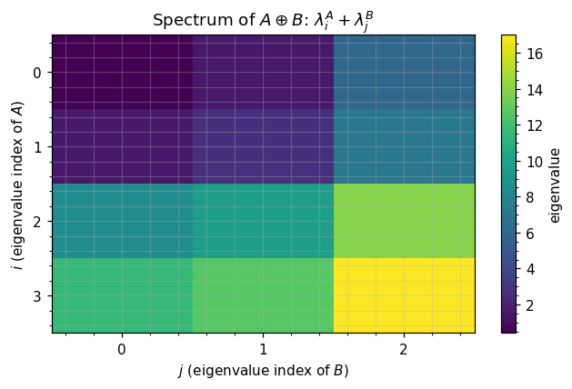
# Visualize spectrum as outer-sum heatmap
fig, ax = plt.subplots(figsize=(6, 4))
heat = lambda_A[:, None] + lambda_B[None, :]
im = ax.imshow(heat, cmap="viridis", aspect="auto")
ax.set_xticks(range(len(lambda_B)))
ax.set_yticks(range(len(lambda_A)))
ax.set_xlabel(r"$j$ (eigenvalue index of $B$)")
ax.set_ylabel(r"$i$ (eigenvalue index of $A$)")
ax.set_title(r"Spectrum of $A\oplus B$: $\lambda^A_i + \lambda^B_j$")
plt.colorbar(im, ax=ax, label="eigenvalue")
plt.tight_layout()
plt.show()

max eigenvalue mismatch : 1.07e-14
first 6 sum-eigs        : [0.42669084 1.56075562 1.58988744 2.72395222 5.91979167 7.05385645]
first 6 direct eigs     : [0.42669084 1.56075562 1.58988744 2.72395222 5.91979167 7.05385645]

3. KroneckerSum solve in $O(n_a^3 + n_b^3)$ ¶

Per eq. ((4)), the solve is three steps:

Project $b$ into the joint eigenbasis: $\tilde b = (Q_A\otimes Q_B)^\top b$ .
Element-wise divide by $\lambda^A_i + \lambda^B_j$ .
Project back: $x = (Q_A\otimes Q_B)\,\tilde x$ .

Steps 1 and 3 are Kronecker-matvecs at $O(n_a n_b(n_a+n_b))$ . Step 2 is element-wise. The dominant cost is the two factor eigh calls.

This is the same scaling as a Kronecker product solve — additive separation costs no more than multiplicative.

# Manual solve through the eigenbasis (mirrors what a structured solver would do)
def kron_sum_solve(A_mat, B_mat, b):
    la, QA = jnp.linalg.eigh(A_mat)
    lb, QB = jnp.linalg.eigh(B_mat)
    n_a, n_b = la.shape[0], lb.shape[0]
    # rotate b into joint eigenbasis: vec(QB^T X QA), where X = mat(b)
    X = einx.id("(a b) -> b a", b, a=n_a, b=n_b)
    X_rot = QB.T @ X @ QA
    # divide by sum of spectra
    denom = la[None, :] + lb[:, None]
    Y_rot = X_rot / denom
    # rotate back
    Y = QB @ Y_rot @ QA.T
    return einx.id("b a -> (a b)", Y)

b = jax.random.normal(jax.random.PRNGKey(3), (12,))
x_struct = kron_sum_solve(A_mat, B_mat, b)
x_dense  = jnp.linalg.solve(KS_dense, b)
print(f"solve error : {jnp.linalg.norm(x_struct - x_dense):.2e}")

# logdet via the spectrum (one log-sum, no Cholesky)
logdet_struct = jnp.sum(jnp.log(lambda_A[:, None] + lambda_B[None, :]))
logdet_dense  = jnp.linalg.slogdet(KS_dense)[1]
print(f"logdet error: {abs(logdet_struct - logdet_dense):.2e}")

solve error : 8.99e-15

logdet error: 7.11e-15

4. `SumKronecker` — superposition of two Kronecker products¶

A different beast. Now we have two Kronecker products and we add them:

M = A_1\otimes B_1 \;+\; A_2\otimes B_2

((5))

The canonical case is multi-output GPs with correlated tasks: $K_{\mathrm{task}}\otimes K_{\mathrm{spatial}} + \sigma^2 I_{\mathrm{task}}\otimes I_{\mathrm{spatial}}$ . Or signal-plus-noise on a tensor grid. Or any covariance where two distinct Kronecker layers superpose.

Matvec is the obvious sum of Kronecker matvecs — cost $2 \cdot O(n_a n_b (n_a+n_b))$ , twice that of a single Kronecker. Solve and logdet are the hard part: in general $A_1, A_2$ do not share eigenvectors, so we cannot simultaneously diagonalize and the spectrum is not a tidy sum or outer-product.

ks_keys = jax.random.split(jax.random.PRNGKey(10), 4)
A1 = psd_op(random_psd(ks_keys[0], 4))
B1 = psd_op(random_psd(ks_keys[1], 3))
A2 = psd_op(random_psd(ks_keys[2], 4))
B2 = psd_op(random_psd(ks_keys[3], 3))

SK = SumKronecker(Kronecker(A1, B1), Kronecker(A2, B2))
SK_dense = jnp.kron(A1.as_matrix(), B1.as_matrix()) + jnp.kron(A2.as_matrix(), B2.as_matrix())

v = jax.random.normal(jax.random.PRNGKey(11), (12,))
print(f"matvec error : {jnp.linalg.norm(SK.mv(v) - SK_dense @ v):.2e}")

# Are A1 and A2 jointly diagonalizable? Compute their commutator.
A1m, A2m = A1.as_matrix(), A2.as_matrix()
comm = A1m @ A2m - A2m @ A1m
print(f"||[A1, A2]||  : {jnp.linalg.norm(comm):.4f}  (non-zero → no shared eigenbasis)")

matvec error : 3.02e-14
||[A1, A2]||  : 35.6242  (non-zero → no shared eigenbasis)

5. The joint-eigenbasis-of-pair-2 trick¶

gaussx’s SumKronecker.eigendecompose() uses a hybrid approach:

Eigendecompose the second pair: $A_2 = Q_C \Lambda_C Q_C^\top$ , $B_2 = Q_D \Lambda_D Q_D^\top$ . Cost: $O(n_a^3 + n_b^3)$ .
Rotate the first pair into that basis: $\tilde A_1 = Q_C^\top A_1 Q_C$ , $\tilde B_1 = Q_D^\top B_1 Q_D$ . Cost: $O(n_a^3 + n_b^3)$ .
Form the rotated full matrix $\tilde A_1 \otimes \tilde B_1 + \mathrm{diag}(\lambda^C_i \lambda^D_j)$ — an $n_a n_b\times n_a n_b$ matrix — and call eigh. Cost: $O((n_a n_b)^3)$ .

The third step is the bottleneck. Unlike KroneckerSum, we cannot avoid a dense pass on the full $N=n_a n_b$ matrix. The trick only buys us:

A symmetric form for eigh (the rotation makes $A_2\otimes B_2$ purely diagonal so the second pair contributes only to the diagonal).
Cheaper structural inheritance (the eigendecomposition is computed once and reused for solve, logdet, and matrix square root).

SumKronecker is intended for moderate factor sizes — typical multi-output GPs with task dimension $\leq 10$ . Past that, you need iterative Krylov solvers (1.D) or alternative parameterizations.

# Verify gaussx's SumKronecker.eigendecompose
evals, Q = SK.eigendecompose()
recon = Q @ jnp.diag(evals) @ Q.T
print(f"eigendecomp residual : {jnp.linalg.norm(recon - SK_dense):.2e}")
print(f"logdet via eigs      : {float(jnp.sum(jnp.log(evals))):.6f}")
print(f"logdet ref           : {float(jnp.linalg.slogdet(SK_dense)[1]):.6f}")

# Solve through the eigendecomposition
b = jax.random.normal(jax.random.PRNGKey(12), (12,))
x_eig = Q @ ((Q.T @ b) / evals)
x_ref = jnp.linalg.solve(SK_dense, b)
print(f"solve error via eigs : {jnp.linalg.norm(x_eig - x_ref):.2e}")

eigendecomp residual : 1.07e-13
logdet via eigs      : 27.528890
logdet ref           : 27.528890
solve error via eigs : 1.97e-14

6. Cost & structure comparison¶

Side-by-side, with $N = n_a n_b$ :

Aspect	`Kronecker` $A\otimes B$	`KroneckerSum` $A\oplus B$	`SumKronecker` $A_1\otimes B_1 + A_2\otimes B_2$
Storage	$n_a^2 + n_b^2$	$n_a^2 + n_b^2$	$2(n_a^2 + n_b^2)$
Matvec	$O(N(n_a + n_b))$	$O(N(n_a + n_b))$	$2\cdot O(N(n_a + n_b))$
Spectrum	$\lambda^A_i \lambda^B_j$	$\lambda^A_i + \lambda^B_j$	no closed form
Solve / logdet	$O(n_a^3 + n_b^3)$	$O(n_a^3 + n_b^3)$	$O(N^3)$ via eigh on $\tilde A_1\otimes\tilde B_1 + \mathrm{diag}$
Constructor	`Kronecker(A, B)`	`KroneckerSum(A, B)`	`SumKronecker(Kronecker(A1,B1), Kronecker(A2,B2))`

The two takeaways:

KroneckerSum is essentially free — same asymptotic cost as a single Kronecker product, including a clean closed-form spectrum.
SumKronecker is moderate-only — the cubic-in- $N$ inner eigh is the price of not having a shared eigenbasis. Use it when $N \lesssim$ a few thousand (multi-output GP with small task dimension); reach for iterative methods otherwise.

7. Solve cost: KroneckerSum vs SumKronecker¶

Theoretical FLOP curves for the eigendecomposition-based solve, sweeping $N = n^2$ (square layout $n_a = n_b = n$ ). KroneckerSum scales as $O(n^3) = O(N^{3/2})$ ; SumKronecker as $O(N^3)$ . Plot is log–log so the slopes are exactly the asymptotic exponents.

ns = np.array([4, 8, 16, 32, 64])
Ns = ns**2

kron_sum_solve_flops    = 2 * (1/3) * ns**3                      # two eigh calls of size n
sum_kron_eig_flops       = 2 * (1/3) * ns**3 + (1/3) * Ns**3     # two factor eighs + dense (n^2)^3 eigh
dense_solve_flops        = (1/3) * Ns**3                          # full Cholesky on N=n^2

fig, ax = plt.subplots(figsize=(7, 5))
ax.loglog(Ns, kron_sum_solve_flops, "C2-",  marker="^", label="KroneckerSum solve")
ax.loglog(Ns, sum_kron_eig_flops,   "C0--", marker="s", label="SumKronecker eigendecomp + solve")
ax.loglog(Ns, dense_solve_flops,    "C3:",  marker="o", label="dense Cholesky baseline")
ax.set_xlabel(r"$N = n_a n_b$ (square layout)")
ax.set_ylabel("FLOPs (theoretical)")
ax.set_title("Solve cost: separable vs superposed Kronecker structure")
ax.legend(loc="upper left")
plt.tight_layout()
plt.show()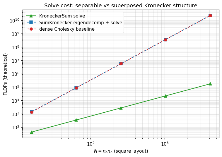

8. Which one do I want?¶

A simple decision rule when you build a covariance with Kronecker-shaped pieces:

Pattern in your covariance	Reach for
“ $A$ acts on rows, $B$ acts on columns, contributions add” (separable PDE / GMRF)	`KroneckerSum(A, B)`
“Kernel on a tensor grid times a coregionalization matrix”	`Kronecker(K_task, K_space)`
“Kernel times correlation plus iid noise on a tensor grid”	`SumKronecker(Kronecker(K_task, K_space), σ²·Kronecker(I, I))`
“Two independent Kronecker layers superposed” (multi-output, multi-fidelity)	`SumKronecker(...)`
“Three or more Kronecker layers”	iterative methods — see 1.E (SLQ logdet, BBMM)

The naming is admittedly cruel — “Kronecker sum” means $A\otimes I + I\otimes B$ in linear-algebra texts, but a “sum of Kroneckers” reads like the same thing in plain English. In gaussx, the operator names track the linear-algebra convention: KroneckerSum = $A\oplus B$ , SumKronecker = $\sum_k A_k\otimes B_k$ . When in doubt, check the eigendecomposition: if the spectrum is a tidy outer-sum of two factor spectra, you have a KroneckerSum. If not, you have a SumKronecker.

The rest of Part 1 fills in the remaining structured leaves (Toeplitz, BlockTriDiag, MaskedOperator) and then 1.7 explains how the kronecker_sum_tag attached on construction lets gaussx’s primitives dispatch through any of these forms automatically.