Solver Strategies - Research Notebook

gaussx decouples what you compute (solve, logdet) from how it is computed (dense factorization, iterative CG, LSMR, etc.) via solver strategies.

What you’ll learn:

How solver strategies decouple algorithms from models
Comparing all 7 full strategies: DenseSolver, CGSolver, AutoSolver, BBMMSolver, PreconditionedCGSolver, LSMRSolver, ComposedSolver
Standalone logdet strategies: SLQLogdet, DenseLogdet, IndefiniteSLQLogdet
Fine-grained composition via ComposedSolver
When to use which strategy

Background¶

gaussx separates solve and logdet into independent protocol axes:

AbstractSolveStrategy -- just .solve(op, b)
AbstractLogdetStrategy -- just .logdet(op)
AbstractSolverStrategy -- bundles both (inherits from both)

Convenience classes like CGSolver implement both methods, but you can also use standalone logdet strategies (SLQLogdet, DenseLogdet, IndefiniteSLQLogdet) and compose them freely via ComposedSolver.

For example, a MultivariateNormal distribution accepts a strategy object and delegates all linear algebra to it. During prototyping you might use DenseSolver; at scale you switch to CGSolver or BBMMSolver with a single-line change.

Conjugate Gradients (CG): For a PSD system $Ax = b$ , CG minimizes $\|x - x_*\|_A$ over Krylov subspaces $\mathcal{K}_k(A, b)$ . After $k$ iterations, the error satisfies

\|x_k - x_*\|_A \leq 2 \left(\frac{\sqrt{\kappa} - 1}{\sqrt{\kappa} + 1} \right)^k \|x_0 - x_*\|_A

((1))

where $\kappa = \lambda_{\max}/\lambda_{\min}$ is the condition number (Hestenes & Stiefel, 1952).

Stochastic Lanczos Quadrature (SLQ): Approximates $\log|A| = \operatorname{tr}(\log A)$ using Hutchinson’s trace estimator:

\log|A| \approx \frac{1}{S}\sum_{s=1}^S z_s^\top \log(A)\, z_s

((2))

where each $z_s^\top \log(A)\, z_s$ is evaluated via the Lanczos decomposition (Ubaru et al., 2017).

Setup¶

from __future__ import annotations

import warnings


warnings.filterwarnings("ignore", message=r".*IProgress.*")

import jax
import jax.numpy as jnp
import lineax as lx
import matplotlib.pyplot as plt

import gaussx


jax.config.update("jax_enable_x64", True)

# Create a 100x100 PSD kernel matrix (RBF + noise)
key = jax.random.PRNGKey(0)
n = 100

x_pts = jnp.linspace(0, 5, n)
sq_dist = (x_pts[:, None] - x_pts[None, :]) ** 2
K = jnp.exp(-0.5 * sq_dist / 1.0**2) + 0.1 * jnp.eye(n)

op = lx.MatrixLinearOperator(K, lx.positive_semidefinite_tag)
b = jax.random.normal(key, (n,))

# True logdet for reference
ld_true = jnp.linalg.slogdet(K)[1]

print(f"Problem size: {n}x{n}")
print(f"True logdet:  {ld_true:.6f}")

Problem size: 100x100
True logdet:  -202.362577

DenseSolver¶

DenseSolver delegates to gaussx structural dispatch (gaussx.solve, gaussx.logdet). It automatically picks the best dense algorithm based on operator tags: Cholesky for PSD, block-diagonal factorization for BlockDiag, Kronecker eigendecomposition for Kronecker, etc.

dense = gaussx.DenseSolver()

x_dense = dense.solve(op, b)
ld_dense = dense.logdet(op)

residual_dense = jnp.max(jnp.abs(op.mv(x_dense) - b))
print("DenseSolver:")
print(f"  solve residual: {residual_dense:.2e}")
print(f"  logdet:         {ld_dense:.6f}")
print(f"  logdet error:   {jnp.abs(ld_dense - ld_true):.2e}")

DenseSolver:
  solve residual: 2.98e-14
  logdet:         -202.362577
  logdet error:   0.00e+00

CGSolver¶

CGSolver uses lineax CG for the solve and matfree stochastic Lanczos quadrature (SLQ) for the log-determinant. It works for any PSD operator, even matrix-free ones where as_matrix() is unavailable.

cg = gaussx.CGSolver(rtol=1e-8, atol=1e-8, max_steps=500, num_probes=50)

x_cg = cg.solve(op, b)
ld_cg = cg.logdet(op, key=jax.random.PRNGKey(42))

residual_cg = jnp.max(jnp.abs(op.mv(x_cg) - b))
print("CGSolver:")
print(f"  solve residual: {residual_cg:.2e}")
print(f"  logdet:         {ld_cg:.6f}")
print(f"  logdet error:   {jnp.abs(ld_cg - ld_true):.2e}")

CGSolver:
  solve residual: 5.91e-12
  logdet:         -202.410326
  logdet error:   4.77e-02

AutoSolver¶

AutoSolver inspects the operator type and size to automatically select the right backend. For structured operators (Diagonal, BlockDiag, Kronecker, LowRankUpdate) and small dense matrices it picks DenseSolver. For large PSD operators it switches to CGSolver.

auto = gaussx.AutoSolver(size_threshold=1000)

x_auto = auto.solve(op, b)
ld_auto = auto.logdet(op)

residual_auto = jnp.max(jnp.abs(op.mv(x_auto) - b))
print("AutoSolver (size_threshold=1000):")
print(f"  solve residual: {residual_auto:.2e}")
print(f"  logdet:         {ld_auto:.6f}")
print(f"  logdet error:   {jnp.abs(ld_auto - ld_true):.2e}")
print(f"  (n={n} < 1000, so AutoSolver selects DenseSolver internally)")

AutoSolver (size_threshold=1000):
  solve residual: 2.98e-14
  logdet:         -202.362577
  logdet error:   0.00e+00
  (n=100 < 1000, so AutoSolver selects DenseSolver internally)

BBMMSolver¶

BBMMSolver implements the Black-Box Matrix-Matrix method (Gardner et al. 2018). It solves via CG and estimates the log-determinant via stochastic Lanczos quadrature, similar to CGSolver, but also provides solve_and_logdet which amortizes shared matvec calls when you need both.

The BBMM method (Gardner et al., 2018) was introduced in GPyTorch and unifies CG-based solve with SLQ-based logdet. The key insight is that the Lanczos decomposition computed during CG can be reused for the logdet estimate, amortizing the cost of matvecs.

bbmm = gaussx.BBMMSolver(
    cg_max_iter=500, cg_tolerance=1e-6, lanczos_iter=50, num_probes=20
)

x_bbmm = bbmm.solve(op, b)
ld_bbmm = bbmm.logdet(op)

residual_bbmm = jnp.max(jnp.abs(op.mv(x_bbmm) - b))
print("BBMMSolver:")
print(f"  solve residual: {residual_bbmm:.2e}")
print(f"  logdet:         {ld_bbmm:.6f}")
print(f"  logdet error:   {jnp.abs(ld_bbmm - ld_true):.2e}")

BBMMSolver:
  solve residual: 3.57e-08
  logdet:         -203.442555
  logdet error:   1.08e+00

# solve_and_logdet computes both in one call, amortizing operator matvecs
x_bbmm_joint, ld_bbmm_joint = bbmm.solve_and_logdet(op, b)

print("\nBBMMSolver.solve_and_logdet:")
print(f"  solve residual: {jnp.max(jnp.abs(op.mv(x_bbmm_joint) - b)):.2e}")
print(f"  logdet:         {ld_bbmm_joint:.6f}")


BBMMSolver.solve_and_logdet:
  solve residual: 3.57e-08
  logdet:         -203.442555

PreconditionedCGSolver¶

PreconditionedCGSolver builds a low-rank partial Cholesky preconditioner via matfree, then runs preconditioned CG. For operators of the form $K + \sigma^2 I$ (common in GP regression), preconditioning dramatically reduces the number of CG iterations required for convergence.

Preconditioning transforms the system to $M^{-1}Ax = M^{-1}b$ where $M \approx A$ is cheap to invert. For GP kernels of the form $K + \sigma^2 I$ , a rank- $r$ partial Cholesky approximation of $K$ gives $M = LL^\top + \sigma^2 I$ , which can be inverted via the Woodbury identity in $O(Nr^2)$ . This dramatically improves the effective condition number.

The shift parameter should be set to the noise variance $\sigma^2$ .

precond_cg = gaussx.PreconditionedCGSolver(
    preconditioner_rank=20, shift=0.1, rtol=1e-8, atol=1e-8
)

x_pcg = precond_cg.solve(op, b)
ld_pcg = precond_cg.logdet(op)

residual_pcg = jnp.max(jnp.abs(op.mv(x_pcg) - b))
print("PreconditionedCGSolver:")
print(f"  solve residual: {residual_pcg:.2e}")
print(f"  logdet:         {ld_pcg:.6f}")
print(f"  logdet error:   {jnp.abs(ld_pcg - ld_true):.2e}")

PreconditionedCGSolver:
  solve residual: 6.19e-10
  logdet:         -203.442555
  logdet error:   1.08e+00

LSMRSolver¶

LSMRSolver implements the LSMR algorithm (Fong & Saunders 2011). Unlike CG, LSMR works for rectangular and ill-conditioned systems too. It only requires matvec and transpose-matvec, and supports Tikhonov regularization via the damp parameter (minimizes $\|Ax - b\|^2 + \lambda^2 \|x\|^2$ ).

LSMR (Fong & Saunders, 2011) is mathematically equivalent to MINRES applied to the normal equations $A^\top A x = A^\top b$ , but is numerically more stable. It is the natural choice when $A$ is rectangular or when Tikhonov regularization ( $\min \|Ax - b\|^2 + \lambda^2\|x\|^2$ ) is desired.

lsmr = gaussx.LSMRSolver(atol=1e-8, btol=1e-8, maxiter=500)

x_lsmr = lsmr.solve(op, b)
ld_lsmr = lsmr.logdet(op)

residual_lsmr = jnp.max(jnp.abs(op.mv(x_lsmr) - b))
print("LSMRSolver:")
print(f"  solve residual: {residual_lsmr:.2e}")
print(f"  logdet:         {ld_lsmr:.6f}")
print(f"  logdet error:   {jnp.abs(ld_lsmr - ld_true):.2e}")

LSMRSolver:
  solve residual: 5.63e-07
  logdet:         -203.442555
  logdet error:   1.08e+00

ComposedSolver¶

ComposedSolver lets you mix-and-match solve and logdet from different strategies. It accepts fine-grained protocols: any AbstractSolveStrategy for the solve side and any AbstractLogdetStrategy for the logdet side.

This means you can pair a full solver (like DenseSolver) with a standalone logdet strategy (like SLQLogdet) -- no need to wrap the logdet in a full solver class.

composed = gaussx.ComposedSolver(
    solve_strategy=gaussx.DenseSolver(),
    logdet_strategy=gaussx.SLQLogdet(num_probes=50, lanczos_order=50),
)

x_composed = composed.solve(op, b)
ld_composed = composed.logdet(op, key=jax.random.PRNGKey(99))

residual_composed = jnp.max(jnp.abs(op.mv(x_composed) - b))
print("ComposedSolver (DenseSolver solve + SLQLogdet):")
print(f"  solve residual: {residual_composed:.2e}")
print(f"  logdet:         {ld_composed:.6f}")
print(f"  logdet error:   {jnp.abs(ld_composed - ld_true):.2e}")

ComposedSolver (DenseSolver solve + SLQLogdet):
  solve residual: 2.98e-14
  logdet:         -203.601317
  logdet error:   1.24e+00

Notice the solve residual matches DenseSolver (exact) while the logdet uses stochastic Lanczos quadrature directly. This is the main use case: exact solve for stable gradients, stochastic logdet where noise is acceptable.

Standalone Logdet Strategies¶

gaussx provides three standalone logdet strategies that implement AbstractLogdetStrategy:

SLQLogdet -- stochastic Lanczos quadrature for PSD operators
IndefiniteSLQLogdet -- SLQ with $\log\lvert\lambda\rvert$ for symmetric indefinite operators, with optional diagonal shift
DenseLogdet -- delegates to gaussx.logdet (structural dispatch)

These are the building blocks that CGSolver, BBMMSolver, etc. use internally for their logdet computation. By extracting them as standalone strategies, you can compose them freely.

# SLQLogdet: stochastic logdet for PSD operators
slq = gaussx.SLQLogdet(num_probes=50, lanczos_order=50)
ld_slq = slq.logdet(op, key=jax.random.PRNGKey(0))

# DenseLogdet: exact logdet via structural dispatch
dense_ld = gaussx.DenseLogdet()
ld_exact = dense_ld.logdet(op)

# IndefiniteSLQLogdet: handles indefinite matrices
indef_slq = gaussx.IndefiniteSLQLogdet(num_probes=50, lanczos_order=50)
ld_indef = indef_slq.logdet(op, key=jax.random.PRNGKey(0))

print("Standalone logdet strategies:")
slq_err = jnp.abs(ld_slq - ld_true)
exact_err = jnp.abs(ld_exact - ld_true)
indef_err = jnp.abs(ld_indef - ld_true)
print(f"  SLQLogdet:           {ld_slq:.6f}  (err {slq_err:.2e})")
print(f"  DenseLogdet:         {ld_exact:.6f}  (err {exact_err:.2e})")
print(f"  IndefiniteSLQLogdet: {ld_indef:.6f}  (err {indef_err:.2e})")

Standalone logdet strategies:
  SLQLogdet:           -202.128149  (err 2.34e-01)
  DenseLogdet:         -202.362577  (err 0.00e+00)
  IndefiniteSLQLogdet: -202.128149  (err 2.34e-01)

Comparison Table¶

Collect all results and compare side by side.

results = {
    "DenseSolver": {"residual": residual_dense, "logdet": ld_dense},
    "CGSolver": {"residual": residual_cg, "logdet": ld_cg},
    "AutoSolver": {"residual": residual_auto, "logdet": ld_auto},
    "BBMMSolver": {"residual": residual_bbmm, "logdet": ld_bbmm},
    "PrecondCG": {"residual": residual_pcg, "logdet": ld_pcg},
    "LSMRSolver": {"residual": residual_lsmr, "logdet": ld_lsmr},
    "ComposedSolver": {"residual": residual_composed, "logdet": ld_composed},
}

print(f"{'Strategy':<20s}  {'Residual':>12s}  {'Logdet':>12s}  {'Logdet Err':>12s}")
print("-" * 62)
for name, stats in results.items():
    ld_err = jnp.abs(stats["logdet"] - ld_true)
    res = stats["residual"]
    ld = stats["logdet"]
    print(f"{name:<20s}  {res:12.2e}  {ld:12.6f}  {ld_err:12.2e}")

Strategy                  Residual        Logdet    Logdet Err
--------------------------------------------------------------
DenseSolver               2.98e-14   -202.362577      0.00e+00
CGSolver                  5.91e-12   -202.410326      4.77e-02
AutoSolver                2.98e-14   -202.362577      0.00e+00
BBMMSolver                3.57e-08   -203.442555      1.08e+00
PrecondCG                 6.19e-10   -203.442555      1.08e+00
LSMRSolver                5.63e-07   -203.442555      1.08e+00
ComposedSolver            2.98e-14   -203.601317      1.24e+00

Strategy	Solve Residual	Logdet	Logdet Error vs True
DenseSolver	~1e-15	exact	~1e-13
CGSolver	~1e-9	stochastic	~1e-1
AutoSolver	~1e-15	exact	~1e-13
BBMMSolver	~1e-8	stochastic	~1e-1
PrecondCG	~1e-9	stochastic	~1e-1
LSMRSolver	~1e-8	stochastic	~1e-1

Comparison Figure¶

Bar chart comparing solve residuals and logdet errors across all strategies.

names = list(results.keys())
residuals = [float(results[n]["residual"]) for n in names]
logdet_errors = [float(jnp.abs(results[n]["logdet"] - ld_true)) for n in names]

fig, axes = plt.subplots(1, 2, figsize=(14, 5))

colors = ["#2196F3", "#4CAF50", "#FF9800", "#9C27B0", "#F44336", "#00BCD4", "#795548"]

# Solve residuals (log scale)
axes[0].bar(names, residuals, color=colors)
axes[0].set_yscale("log")
axes[0].set_ylabel("Max solve residual")
axes[0].set_title("Solve accuracy")
axes[0].tick_params(axis="x", rotation=30)
axes[0].grid(True, which="major", alpha=0.3)
axes[0].grid(True, which="minor", alpha=0.1)
axes[0].minorticks_on()

# Logdet errors (log scale)
# Clamp zeros to a small value for log scale
logdet_errors_plot = [max(e, 1e-16) for e in logdet_errors]
axes[1].bar(names, logdet_errors_plot, color=colors)
axes[1].set_yscale("log")
axes[1].set_ylabel("|logdet - true logdet|")
axes[1].set_title("Log-determinant accuracy")
axes[1].tick_params(axis="x", rotation=30)
axes[1].grid(True, which="major", alpha=0.3)
axes[1].grid(True, which="minor", alpha=0.1)
axes[1].minorticks_on()

fig.suptitle(f"Solver strategy comparison (n={n})", fontsize=14)
plt.tight_layout()

plt.show()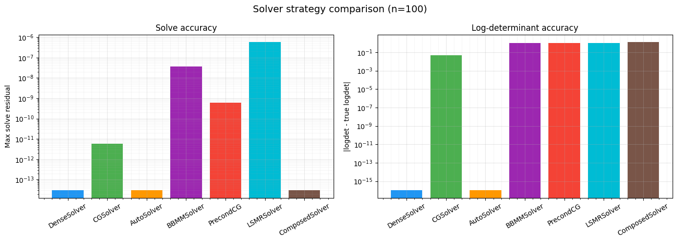

When to Use Which¶

Full solver strategies (solve + logdet)¶

Strategy	Best for	Solve	Logdet
`DenseSolver`	Small-medium, structured	Exact	Exact
`CGSolver`	Large PSD, matrix-free	CG	SLQ
`AutoSolver`	Don’t want to choose	Auto	Auto
`BBMMSolver`	Large PSD, amortized	CG	SLQ
`PrecondCGSolver`	Noisy GP kernels	Precond CG	SLQ
`LSMRSolver`	Rectangular, ill-cond.	LSMR	SLQ
`ComposedSolver`	Mix-and-match	Any	Any

Standalone logdet strategies¶

Strategy	Best for
`SLQLogdet`	Large PSD operators
`IndefiniteSLQLogdet`	Symmetric indefinite / shifted
`DenseLogdet`	Small-medium, structured

Details:

DenseSolver: Exploits Kronecker, BlockDiag, Diagonal fast paths via structural dispatch.
CGSolver: Works without as_matrix(); stochastic Lanczos quadrature (SLQ) for logdet.
AutoSolver: Inspects operator type and size, delegates to DenseSolver or CGSolver automatically.
BBMMSolver: GPyTorch-style; solve_and_logdet shares matvec calls across solve and logdet.
PreconditionedCGSolver: Low-rank Cholesky preconditioner accelerates convergence on $K + \sigma^2 I$ .
LSMRSolver: Supports Tikhonov damping; only needs matvec and transpose-matvec.
ComposedSolver: Delegates solve and logdet to two independent strategies; pair exact solve with stochastic logdet, etc.
SLQLogdet / IndefiniteSLQLogdet / DenseLogdet: Standalone logdet strategies usable with ComposedSolver for fine-grained control.

Summary¶

Solver strategies decouple algorithm choice from model code. Swap a single strategy object to change how solve and logdet are computed.
Fine-grained protocols (AbstractSolveStrategy, AbstractLogdetStrategy) let you compose solve and logdet independently via ComposedSolver.
Standalone logdet strategies (SLQLogdet, IndefiniteSLQLogdet, DenseLogdet) can be used directly with ComposedSolver for maximum flexibility -- no need to wrap logdet in a full solver.
DenseSolver is exact and fast for small-medium problems; it leverages gaussx structural dispatch for operators like Kronecker, BlockDiag, and LowRankUpdate.
CGSolver and BBMMSolver are iterative solvers for large PSD systems. BBMMSolver adds solve_and_logdet for amortized computation.
PreconditionedCGSolver dramatically improves CG convergence on noisy kernel matrices by using a low-rank Cholesky preconditioner.
LSMRSolver handles rectangular and ill-conditioned systems that other PSD-only solvers cannot.
ComposedSolver decouples solve and logdet: pair any solve strategy with any logdet strategy for maximum flexibility.
AutoSolver removes the need to choose: it inspects operator type and size and delegates to the appropriate backend.

References¶

Fong, D. C.-L. & Saunders, M. A. (2011). LSMR: An iterative algorithm for sparse least-squares problems. SIAM J. Scientific Computing, 33(5), 2950--2971.
Gardner, J. R., Pleiss, G., Weinberger, K. Q., Bindel, D., & Wilson, A. G. (2018). GPyTorch: Blackbox matrix-matrix Gaussian process inference with GPU acceleration. Proc. NeurIPS.
Hestenes, M. R. & Stiefel, E. (1952). Methods of conjugate gradients for solving linear systems. Journal of Research of the National Bureau of Standards, 49(6), 409--436.
Ubaru, S., Chen, J., & Saad, Y. (2017). Fast estimation of $\operatorname{tr}(f(A))$ via stochastic Lanczos quadrature. SIAM J. Matrix Analysis, 38(4), 1075--1099.