Lazy operator algebra — Sum, Scaled, Product

Notebook 1.1 toured the leaf operators: Diagonal, Kronecker, BlockDiag, LowRankUpdate. Real covariances are not leaves — they are expressions. A noisy GP kernel is $\sigma^2 K + \tau^2 I$ . A posterior covariance is $K - K_{*X} K_{XX}^{-1} K_{X*}$ . A whitened cross-term is $L^{-1} K L^{-\top}$ . Each one is a combination of leaves under sum, scalar multiply, and matrix product.

The temptation is to just call .as_matrix() on the leaves and add them together. That works, and it throws away every dollar of structure you bought in 1.1: the moment you materialize $\sigma^2 K_{\mathrm{kron}}$ , its $n^2 + m^2$ parameters explode into $N^2$ entries, and the next call costs $O(N^3)$ instead of $O(N^{3/2})$ .

gaussx provides three lazy combinators — SumOperator, ScaledOperator, ProductOperator — that defer materialization. They store pointers to the operands and a recipe for matvec; they never form the combined matrix unless someone explicitly asks for it. The leaves keep their structural cost; the tree composes.

What you will see by the end:

The matvec rules for sum / scaled / product, and why they preserve leaf cost.
How structural tags propagate: when does a sum stay symmetric? when does a scaled operator stay PSD? (Spoiler: less often than you would expect — gaussx is conservative on purpose.)
A worked composition: $\sigma^2 (K_x \otimes K_y) + \tau^2 I$ assembled lazily on a $32\times 32$ grid.
The “common idioms” cheatsheet — six expressions every GP user writes, paired with the lazy operator that keeps them cheap.
The sharp edges: $AB$ is not generally symmetric or PSD even when both factors are.

By the end you should write covariance arithmetic by operator algebra, not by jnp.zeros((N, N)) followed by accumulation.

0. Where these structures show up in geoscience¶

Lazy algebra is what lets you write down realistic geophysical covariances without paying $O(N^2)$ to materialize them:

Signal + noise: $\sigma^2 K_{\mathrm{rbf}} + \tau^2 I$ — every regression on satellite retrievals, gridded reanalyses, or station data. The kernel captures spatial correlation; the diagonal captures retrieval / instrument noise. Lazy keeps the kernel structured.
Additive kernel decomposition: $K_{\mathrm{trend}} + K_{\mathrm{seasonal}} + K_{\mathrm{residual}}$ — the classic Mauna Loa CO₂ decomposition (Rasmussen & Williams 2006), and any climate-time-series model that separates secular trend, annual cycle, and short-term variability.
Heteroscedastic noise: $K_{XX} + \mathrm{diag}(\sigma_i^2)$ — sparse field campaigns where each observation site has its own precision (Argo float vs ship CTD vs satellite). Sum(K, DiagonalLinearOperator) keeps both sides cheap.
Spacetime separable + iid noise: $\sigma^2 (K_{\mathrm{space}} \otimes K_{\mathrm{time}}) + \tau^2 I$ — any gridded reanalysis, ocean colour series, ENSO prediction. Lazy keeps the Kronecker factor unmaterialized; we’ll see in 1.3 that the eigendecomposition of this composite is also closed-form.
Scaled kernel for output magnitude: $\sigma_f^2 k(\cdot,\cdot)$ where $\sigma_f^2$ is the signal variance — this is a one-cell example of ScaledOperator and shows up in every GP regression model.
Cross-covariance for prediction: $K_{*X} K_{XX}^{-1}$ — the predictive-mean machinery for any geophysical interpolation. The inverse stays implicit (Cholesky factor); the cross-product is lazy Product.

The lesson: writing covariances by operator algebra on top of structured leaves is what makes regional climate / ocean / atmosphere models tractable on commodity GPUs.

from __future__ import annotations

import warnings
warnings.filterwarnings("ignore", message=r".*IProgress.*")

import einx
import jax
import jax.numpy as jnp
import lineax as lx
import matplotlib.pyplot as plt
import numpy as np
from gaussx import (
    Kronecker,
    ProductOperator,
    ScaledOperator,
    SumOperator,
    logdet,
    solve,
)

jax.config.update("jax_enable_x64", True)
KEY = jax.random.PRNGKey(0)
plt.rcParams.update({
    "figure.dpi": 110,
    "axes.grid": True,
    "axes.grid.which": "both",
    "xtick.minor.visible": True,
    "ytick.minor.visible": True,
    "grid.alpha": 0.3,
})

def psd_op(M):
    return lx.MatrixLinearOperator(M, lx.positive_semidefinite_tag)

def random_psd(key, n, jitter=1e-3):
    A = jax.random.normal(key, (n, n))
    return A @ A.T + jitter * jnp.eye(n)

1. Why lazy?¶

Consider a noisy kernel on a $d_1\times d_2$ grid:

M = \sigma^2\,(K_x \otimes K_y) + \tau^2 I_N, \qquad N = d_1 d_2

((1))

If we materialize before adding, we allocate an $N\times N$ array — $N^2$ floats — and lose the Kronecker factorization forever. Subsequent matvec costs $O(N^2)$ , solve costs $O(N^3)$ .

If we keep $M$ lazy, the operator carries:

a pointer to $K_x$ ( $d_1^2$ floats),
a pointer to $K_y$ ( $d_2^2$ floats),
two scalars $\sigma^2, \tau^2$ .

Total storage: $d_1^2 + d_2^2 + O(1)$ instead of $N^2 = d_1^2 d_2^2$ . Matvec dispatches to each leaf and stays $O(N(d_1+d_2))$ via the Kronecker vec-trick. Lazy algebra is what turns the leaves of 1.1 into a usable system.

2. `SumOperator` — lazy addition¶

The matvec is the obvious one:

\Big(\sum_k A_k\Big) v = \sum_k A_k\, v

((2))

Cost is the sum of leaf matvec costs. All operands must share input and output shape (they live in the same vector space). gaussx’s tag rules (registered in gaussx._operators.__init__) propagate symmetry / diagonality / PSD only when every operand carries the property:

\mathrm{sym}\!\left(\textstyle\sum_k A_k\right) = \bigwedge_k \mathrm{sym}(A_k), \qquad \mathrm{psd}\!\left(\textstyle\sum_k A_k\right) = \bigwedge_k \mathrm{psd}(A_k)

((3))

This matches the math: a sum of symmetric matrices is symmetric; a sum of PSD matrices is PSD.

kA, kB = jax.random.split(jax.random.PRNGKey(1))
A = psd_op(random_psd(kA, 5))
B = psd_op(random_psd(kB, 5))

S = SumOperator(A, B)
v = jax.random.normal(jax.random.PRNGKey(2), (5,))

# matvec correctness
ref = A.as_matrix() + B.as_matrix()
print(f"matvec error : {jnp.linalg.norm(S.mv(v) - ref @ v):.2e}")

# tag propagation
print(f"is_symmetric        : {lx.is_symmetric(S)}")
print(f"is_positive_semidef : {lx.is_positive_semidefinite(S)}")
print(f"is_diagonal         : {lx.is_diagonal(S)}")

matvec error : 3.20e-15
is_symmetric        : True
is_positive_semidef : True
is_diagonal         : False

3. `ScaledOperator` — lazy scalar multiply¶

Unspectacular but ubiquitous: every kernel hyperparameter $\sigma^2$ rides in front of an operator.

(c A) v = c (A v)

((4))

The tag rules have one nuance worth flagging. Symmetry and diagonality always survive scaling, but PSD does not auto-propagate — gaussx only marks $cA$ as PSD if you pass tags=lx.positive_semidefinite_tag explicitly. The reason is conservative: under JAX tracing, $c$ may be a tracer whose sign isn’t statically known, so the library refuses to claim PSD on faith. If you know $c \geq 0$ (e.g. you parameterize $\sigma^2 = \exp(\log\sigma^2)$ ), pass the tag yourself.

\mathrm{sym}(cA) = \mathrm{sym}(A), \qquad \mathrm{psd}(cA) = \big[c \geq 0 \;\land\; \mathrm{psd}(A)\big]

((5))

# Default: PSD does NOT auto-propagate
Sc_default = ScaledOperator(A, 2.0)
print(f"Scaled(A, 2.0)               is_psd = {lx.is_positive_semidefinite(Sc_default)}  (conservative default)")

# Pass the tag yourself if you know c >= 0
Sc_tagged = ScaledOperator(A, 2.0, tags=lx.positive_semidefinite_tag)
print(f"Scaled(A, 2.0, tags=psd_tag) is_psd = {lx.is_positive_semidefinite(Sc_tagged)}")

# Symmetric still propagates automatically
print(f"Scaled(A, 2.0)               is_sym = {lx.is_symmetric(Sc_default)}")

# Negative scalar: PSD claim would be wrong, so don't tag it
Sc_neg = ScaledOperator(A, -1.0)
M_neg = Sc_neg.as_matrix()
print(f"\nScaled(A, -1.0) eigenvalues : {jnp.linalg.eigvalsh(M_neg)}  (sign-flipped → not PSD)")

Scaled(A, 2.0)               is_psd = False  (conservative default)
Scaled(A, 2.0, tags=psd_tag) is_psd = True
Scaled(A, 2.0)               is_sym = True

Scaled(A, -1.0) eigenvalues : [-1.70065342e+01 -8.70035471e+00 -3.46205666e+00 -6.23756759e-01
 -7.11341880e-03]  (sign-flipped → not PSD)

4. `ProductOperator` — lazy matmul¶

Two operators with matching inner dimension $\mathrm{in}(A) = \mathrm{out}(B)$ compose into a third whose matvec is $A(Bv)$ — never form $AB$ .

(A B) v = A (B v)

((6))

Cost: $\mathrm{matvec}(A) + \mathrm{matvec}(B)$ . No materialization unless you call .as_matrix().

The tag rules are the most conservative of the three because product structure is genuinely fragile:

\mathrm{sym}(AB) \neq \mathrm{sym}(A)\land\mathrm{sym}(B), \qquad \mathrm{psd}(AB) \neq \mathrm{psd}(A)\land\mathrm{psd}(B)

((7))

Two symmetric matrices multiply into a symmetric matrix only when they commute ( $AB = BA$ ). Two PSD matrices multiply into a PSD matrix only in special cases. gaussx therefore requires you to assert these tags via the tags= argument when you know they hold (e.g. $A^\top A$ is always PSD; $L L^\top$ is always PSD).

The next cell shows the gotcha with two PSD operands whose product is neither symmetric nor PSD.

A_mat = jnp.array([[2., 1.], [1., 2.]])
B_mat = jnp.array([[3., 1.], [1., 2.]])
A2 = lx.MatrixLinearOperator(A_mat, lx.positive_semidefinite_tag)
B2 = lx.MatrixLinearOperator(B_mat, lx.positive_semidefinite_tag)

print(f"A is PSD: {lx.is_positive_semidefinite(A2)},  B is PSD: {lx.is_positive_semidefinite(B2)}")
print(f"A eigvals: {jnp.linalg.eigvalsh(A_mat)},  B eigvals: {jnp.linalg.eigvalsh(B_mat)}")

P = ProductOperator(A2, B2)
AB = P.as_matrix()
print(f"\nAB =\n{AB}")
print(f"AB - (AB)^T =\n{AB - AB.T}    (non-zero → AB is NOT symmetric)")
print(f"AB eigenvalues : {jnp.linalg.eigvals(AB)}  (complex / non-real possible in general)")

print(f"\ngaussx tag propagation:")
print(f"  is_symmetric : {lx.is_symmetric(P)}  (correctly refuses to claim)")
print(f"  is_psd       : {lx.is_positive_semidefinite(P)}")

A is PSD: True,  B is PSD: True
A eigvals: [1. 3.],  B eigvals: [1.38196601 3.61803399]


AB =
[[7. 4.]
 [5. 5.]]

AB - (AB)^T =
[[ 0. -1.]
 [ 1.  0.]]    (non-zero → AB is NOT symmetric)

AB eigenvalues : [10.58257569+0.j  1.41742431+0.j]  (complex / non-real possible in general)

gaussx tag propagation:
  is_symmetric : False  (correctly refuses to claim)
  is_psd       : False

5. A worked composition: $\sigma^2 (K_x\otimes K_y) + \tau^2 I$ ¶

The canonical “noisy GP on a tensor-product grid” — assembled with three combinators on top of a Kronecker and an IdentityLinearOperator:

M = SumOperator(
    ScaledOperator(Kronecker(K_x, K_y), sigma2, tags=lx.positive_semidefinite_tag),
    ScaledOperator(lx.IdentityLinearOperator(jax.ShapeDtypeStruct((N,), jnp.float64)), tau2,  tags=lx.positive_semidefinite_tag),
)

We pass the PSD tag on each ScaledOperator because we know $\sigma^2, \tau^2 > 0$ . The SumOperator then propagates PSD into the composite — and a PSD-tagged operator is what gaussx.solve needs to dispatch to Cholesky.

d1, d2 = 8, 6  # grid 8x6 = 48 points
N = d1 * d2

kx, ky = jax.random.split(jax.random.PRNGKey(3))
K_x = psd_op(random_psd(kx, d1))
K_y = psd_op(random_psd(ky, d2))
sigma2, tau2 = 1.5, 0.1

K_kron = Kronecker(K_x, K_y)
I_N = lx.IdentityLinearOperator(jax.ShapeDtypeStruct((N,), jnp.float64))

M_lazy = SumOperator(
    ScaledOperator(K_kron, sigma2, tags=lx.positive_semidefinite_tag),
    ScaledOperator(I_N,    tau2,  tags=lx.positive_semidefinite_tag),
)

# matvec correctness
v = jax.random.normal(jax.random.PRNGKey(4), (N,))
M_dense = sigma2 * jnp.kron(K_x.as_matrix(), K_y.as_matrix()) + tau2 * jnp.eye(N)
print(f"matvec error : {jnp.linalg.norm(M_lazy.mv(v) - M_dense @ v):.2e}")

# tags propagated through the tree
print(f"M is symmetric : {lx.is_symmetric(M_lazy)}")
print(f"M is PSD       : {lx.is_positive_semidefinite(M_lazy)}")

# Storage: leaves only
leaf_floats = K_x.as_matrix().size + K_y.as_matrix().size + 2  # + 2 scalars
print(f"\nLazy storage : {leaf_floats} floats  (K_x + K_y + 2 scalars)")
print(f"Dense storage: {N*N} floats           ({N*N / leaf_floats:.0f}x larger)")

# logdet via the lazy tree:  log|σ² K + τ² I| via det-lemma is non-trivial,
# but a direct Cholesky-on-as_matrix() works. Lazy doesn't (yet) provide a
# closed-form rule for SumOperator(Kronecker, Scaled-Id) — a Woodbury opportunity.
ld = float(logdet(M_lazy))
ld_ref = float(jnp.linalg.slogdet(M_dense)[1])
print(f"\nlogdet(M) lazy : {ld:.6f}")
print(f"logdet(M) dense: {ld_ref:.6f}")
print(f"agreement      : {abs(ld - ld_ref):.2e}")

matvec error : 1.13e-13
M is symmetric : True
M is PSD       : True

Lazy storage : 102 floats  (K_x + K_y + 2 scalars)
Dense storage: 2304 floats           (23x larger)


logdet(M) lazy : 82.616136
logdet(M) dense: 82.616136
agreement      : 0.00e+00

6. What dispatches, and what falls back¶

Lazy algebra preserves matvec cost cheaply, but solve and logdet on a generic SumOperator typically fall back to materialization — as_matrix() followed by Cholesky. That is the right default (correctness over cleverness), but it is also the motivation for the structured solve rules taught later in the chapter:

Composite	Closed-form solve / logdet rule	Notebook
$A + UDV^\top$	Sherman–Morrison–Woodbury, det-lemma	1.B `woodbury_solve`
$A_1\otimes I + I\otimes A_2$	KroneckerSum eigendecomposition	1.3 `kronecker_sum_vs_sum_kronecker`
Block tridiagonal Λ	UDL / forward–backward sweep	1.5 `block_tridiag`
$\sigma^2 K + \tau^2 I$ with eigendecomposable $K$	Diagonalize $K$ once, broadcast $\sigma^2 \lambda + \tau^2$	(3.B)

Everything else: SumOperator hands the matrix to lineax’s default Cholesky. That’s $O(N^3)$ — acceptable for moderate $N$ , prohibitive at scale, and a clear signal you should reach for a structured class instead of generic lazy sum.

7. Tag-propagation tables¶

A short reference for “if I compose, what do I keep?” — exactly mirroring the dispatch rules registered in gaussx._operators.__init__.

7.1 Symmetric¶

Combinator	Rule	Why
`Sum`	$\bigwedge_k \mathrm{sym}(A_k)$	$(A+B)^\top = A^\top + B^\top$
`Scaled`	inherits from operand	$(cA)^\top = c A^\top$
`Product`	only if explicitly tagged	$AB \neq B^\top A^\top$ in general

7.2 Positive semidefinite¶

Combinator	Rule	Why
`Sum`	$\bigwedge_k \mathrm{psd}(A_k)$	$v^\top(A+B)v \geq 0$ if both terms $\geq 0$
`Scaled`	only if explicitly tagged	sign of $c$ not statically known
`Product`	only if explicitly tagged	$AB$ may have complex eigenvalues

7.3 Diagonal¶

Combinator	Rule
`Sum`	$\bigwedge_k \mathrm{diag}(A_k)$
`Scaled`	inherits from operand
`Product`	always `False` (conservative)

The Scaled/Product PSD entries are the ones that catch users — when you build $\sigma^2 K$ and gaussx.solve won’t dispatch to Cholesky, the fix is to add tags=lx.positive_semidefinite_tag because you know $\sigma^2 \geq 0$ and the library can’t infer that under tracing.

8. Storage cost: lazy vs eager¶

The composition $\sigma^2 (K_x\otimes K_y) + \tau^2 I$ on a square $\sqrt N \times \sqrt N$ grid: lazy keeps two factor matrices of size $\sqrt N$ each, eager materializes the full $N\times N$ . Plotted directly from the analytic formula, log–log.

Ns = np.array([64, 256, 1024, 4096, 16384, 65536])
sqrtN = np.sqrt(Ns).astype(int)
lazy_floats  = 2 * sqrtN**2 + 2          # K_x + K_y + 2 scalars
eager_floats = Ns**2

fig, ax = plt.subplots(figsize=(7, 5))
ax.loglog(Ns, eager_floats, "C3-",  marker="o", label="eager: dense $N\\times N$")
ax.loglog(Ns, lazy_floats,  "C2--", marker="s", label="lazy: $K_x + K_y$ + 2 scalars")
ax.set_xlabel("ambient dimension $N$ (square grid)")
ax.set_ylabel("storage (floats)")
ax.set_title(r"Storage: $\sigma^2 (K_x\otimes K_y) + \tau^2 I$  —  lazy vs eager")
ax.legend(loc="upper left")
plt.tight_layout()
plt.show()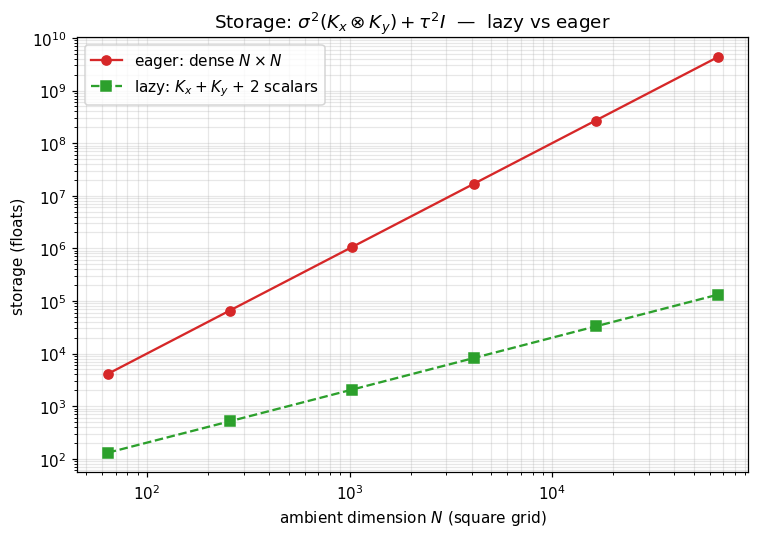

9. Common idioms cheatsheet¶

Six expressions every GP user writes, paired with the lazy form:

Math	Lazy form	Notes
$\sigma^2 K + \tau^2 I$	`Sum(Scaled(K, σ²), Scaled(I, τ²))`	tag both `Scaled` PSD if $\sigma^2, \tau^2 \geq 0$
$K_{XX} + \mathrm{diag}(\sigma_i^2)$	`Sum(K_XX, DiagonalLinearOperator(σ²_vec))`	heteroscedastic noise
$L K L^\top$ (whitening)	`Product(Product(L, K), L.T)`	tag with PSD if $K$ PSD
$K + UU^\top$ (rank- $k$ correction)	use `low_rank_plus_diag` directly	structured leaf, not lazy
$\sigma^2 K_x \otimes K_y + \tau^2 I$	`Sum(Scaled(Kronecker(K_x, K_y), σ²), Scaled(I, τ²))`	the §5 demo
$K_{*X} K_{XX}^{-1}$ (cross-covariance)	precompute $K_{XX}^{-1}$ , then `Product(K_starX, K_inv)`	usually the inv stays lazy via `solve`

The last row is the most common GP-prediction pattern: never form $K_{XX}^{-1}$ explicitly — store it implicitly via a Cholesky factor and apply it through solve / lx.linear_solve. Lazy Product is for the cross-covariance layer that sits on top.

That is the algebra. The next four notebooks (1.3–1.6) introduce structured leaves (KroneckerSum, Toeplitz, BlockTriDiag, MaskedOperator) that the lazy combinators here will glue together; the structural-tag dispatch system is detailed in §10–§13 of 1.1 (operator_basics).