Woodbury Solve Step by Step - Research Notebook

The Woodbury matrix identity turns an $n \times n$ solve into a cheap $k \times k$ solve when the matrix has low-rank structure:

(L + U D V^\top)^{-1} = L^{-1} - L^{-1} U \, C^{-1} \, V^\top L^{-1}

((1))

where $C = D^{-1} + V^\top L^{-1} U$ is the $k \times k$ capacitance matrix.

This notebook walks through each step and shows that gaussx.solve does it automatically.

Background¶

The Woodbury identity (also known as the matrix inversion lemma or Sherman-Morrison-Woodbury formula) is one of the most important identities in computational linear algebra. It appears in:

Sparse GP inference — the Nystrom approximation yields a low-rank + diagonal covariance, and the Woodbury identity turns the $n \times n$ inversion into a $k \times k$ problem where $k \ll n$ .
Kalman filtering — sequential rank-1 updates to the state covariance are applied via the matrix inversion lemma at each time step.
Online learning — rank-1 covariance updates (e.g. recursive least squares) use the Sherman-Morrison special case.
Ridge regression with feature space formulations — the kernel trick relates the $n \times n$ and $p \times p$ solutions through Woodbury.

The identity was first published by Woodbury (1950) and independently by Sherman & Morrison (1950) for the rank-1 case.

from __future__ import annotations

import warnings


warnings.filterwarnings("ignore", message=r".*IProgress.*")

import jax
import jax.numpy as jnp
import matplotlib.pyplot as plt

import gaussx


jax.config.update("jax_enable_x64", True)

Setup¶

We construct $A = \mathrm{diag}(d) + U U^\top$ where $d \in \mathbb{R}^{100}$ and $U \in \mathbb{R}^{100 \times 3}$ (rank 3).

key = jax.random.PRNGKey(0)
k1, k2, k3 = jax.random.split(key, 3)

n, rank = 100, 3
d = jnp.abs(jax.random.normal(k1, (n,))) + 0.5  # positive diagonal
U = jax.random.normal(k2, (n, rank)) * 0.5
b = jax.random.normal(k3, (n,))

# Build operator
sigma = gaussx.low_rank_plus_diag(d, U)
print(f"Operator: diag({n}) + rank-{rank} update")
print(f"  Full matrix size: {n}x{n} = {n**2:,} entries")
print(f"  Low-rank storage: {n} + {n}x{rank} = {n + n * rank:,} entries")

Operator: diag(100) + rank-3 update
  Full matrix size: 100x100 = 10,000 entries
  Low-rank storage: 100 + 100x3 = 400 entries

Step-by-step Woodbury¶

# Step 1: L^{-1} b  (cheap — diagonal solve)
Linv_b = b / d
print("Step 1: L^{-1} b  — diagonal solve, O(n)")

# Step 2: L^{-1} U  (k diagonal solves)
Linv_U = U / d[:, None]
print(f"Step 2: L^{{-1}} U  — {rank} diagonal solves, O(nk)")

# Step 3: Capacitance matrix C = I + U^T L^{-1} U  (k x k)
C = jnp.eye(rank) + U.T @ Linv_U
print(f"Step 3: C = I + U^T L^{{-1}} U  — {rank}x{rank} matrix")

# Step 4: Solve C z = U^T L^{-1} b  (k x k dense solve)
z = jnp.linalg.solve(C, U.T @ Linv_b)
print(f"Step 4: C^{{-1}} (V^T L^{{-1}} b)  — {rank}x{rank} solve")

# Step 5: x = L^{-1} b - L^{-1} U z
x_woodbury = Linv_b - Linv_U @ z
print("Step 5: x = L^{-1} b - L^{-1} U z  — final answer")

Step 1: L^{-1} b  — diagonal solve, O(n)
Step 2: L^{-1} U  — 3 diagonal solves, O(nk)

Step 3: C = I + U^T L^{-1} U  — 3x3 matrix
Step 4: C^{-1} (V^T L^{-1} b)  — 3x3 solve

Step 5: x = L^{-1} b - L^{-1} U z  — final answer

Verify against gaussx.solve¶

x_gaussx = gaussx.solve(sigma, b)
x_dense = jnp.linalg.solve(sigma.as_matrix(), b)

print(f"Woodbury vs dense:  max|diff| = {jnp.max(jnp.abs(x_woodbury - x_dense)):.2e}")
print(f"gaussx  vs dense:   max|diff| = {jnp.max(jnp.abs(x_gaussx - x_dense)):.2e}")
print(f"Woodbury vs gaussx: max|diff| = {jnp.max(jnp.abs(x_woodbury - x_gaussx)):.2e}")

Woodbury vs dense:  max|diff| = 5.55e-15
gaussx  vs dense:   max|diff| = 5.55e-15
Woodbury vs gaussx: max|diff| = 0.00e+00

Matrix determinant lemma¶

Similarly, the logdet decomposes. This follows from the identity

|A + UDV^\top| = |D^{-1} + V^\top A^{-1} U| \cdot |D| \cdot |A|

((2))

which is a direct consequence of the Schur complement determinant identity. Taking logarithms:

\log|A + UDV^\top| = \log|A| + \log|C| + \log|D|

((3))

where $C = D^{-1} + V^\top A^{-1} U$ is the capacitance matrix. In our case ( $D = I$ , $V = U$ ):

ld_gaussx = gaussx.logdet(sigma)
ld_dense = jnp.linalg.slogdet(sigma.as_matrix())[1]

print(f"gaussx logdet:  {ld_gaussx:.6f}")
print(f"dense logdet:   {ld_dense:.6f}")
print(f"match: {jnp.allclose(ld_gaussx, ld_dense, rtol=1e-10)}")

gaussx logdet:  27.039277
dense logdet:   27.039277
match: True

Visualizing the decomposition¶

fig, axes = plt.subplots(1, 4, figsize=(14, 3))

axes[0].imshow(jnp.diag(d[:20]), cmap="Blues", interpolation="nearest")
axes[0].set_title("L = diag(d)\n(first 20x20)")

axes[1].imshow(U[:20], cmap="RdBu", interpolation="nearest", aspect="auto")
axes[1].set_title(f"U\n({n}x{rank}, first 20 rows)")

axes[2].imshow(C, cmap="Blues", interpolation="nearest")
axes[2].set_title(f"C (capacitance)\n({rank}x{rank})")

mat_20 = jnp.abs(sigma.as_matrix()[:20, :20])
axes[3].imshow(mat_20, cmap="Blues", interpolation="nearest")
axes[3].set_title("A = L + UU^T\n(first 20x20)")

for ax in axes:
    ax.set_xticks([])
    ax.set_yticks([])

plt.tight_layout()
plt.show()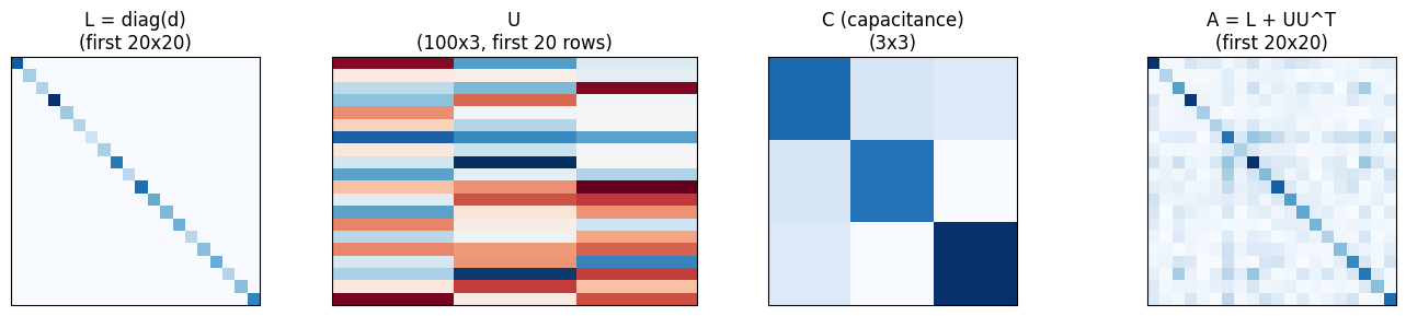

Cost comparison¶

Operation	Dense	Woodbury
Solve	O(n^3)	O(nk^2 + k^3)
Logdet	O(n^3)	O(nk^2 + k^3)
Storage	O(n^2)	O(nk)

For n=100, k=3: dense does ~10^6 ops, Woodbury does ~900.

References¶

Hager, W. W. (1989). Updating the inverse of a matrix. SIAM Review, 31(2), 221--239.
Henderson, H. V. & Searle, S. R. (1981). On deriving the inverse of a sum of matrices. SIAM Review, 23(1), 53--60.
Woodbury, M. A. (1950). Inverting Modified Matrices. Statistical Research Group Memo Report 42, Princeton University.