Masked operators — missing data on a structured grid

Real geophysical datasets are partial. Clouds occlude satellite retrievals; ARGO floats sample a sparse subset of the ocean; tide gauges miss days; ice cores have hiatuses; GPS stations drop out. The kernel covariance over the full regular grid is structured (Toeplitz, Kronecker, block-tridiagonal); the kernel over the observed subset is structureless dense. Materializing the subset throws away every dollar of structure you spent the last five notebooks earning back.

MaskedOperator is the bridge: keep the structured base operator on the full grid, attach boolean row/column masks, and perform every matvec at the base operator’s cost — without ever assembling the dense subset matrix. This is the single most useful operator for working with real environmental data.

0. Where masked operators show up in geoscience¶

The list of geoscience workflows that need exactly this primitive:

The simplest case — subset of a plain MVN: a generic dense covariance $\Sigma\in\mathbb{R}^{N\times N}$ describing some multivariate normal field, and you want the marginal over an observed subset. MaskedOperator(MatrixLinearOperator(Σ), mask, mask) returns $\Sigma[r][:,r]$ as an operator without copying — useful for parameter tying across many masks (cross-validation folds, leave-one-out diagnostics, multiple cloud frames against the same prior).
Markovian GPs with missing observations: Matérn-1/2, -3/2, -5/2 GPs in time as state-space models have a BlockTriDiag precision on a regular grid. Real geophysical timeseries — GPS, tide gauges, soil-moisture probes, eddy-covariance flux towers — drop observations regularly. MaskedOperator(BlockTriDiag, time_mask, time_mask) keeps the $O(N d^3)$ banded prior on the full timeline and selects observed timesteps cheaply. This is the standard pattern for state-space GP regression with gaps.
Cloud-masked satellite retrievals: SST (MODIS, AVHRR, VIIRS), ocean colour / chlorophyll, atmospheric CO₂ (OCO-2, GOSAT), surface temperature. The covariance on the underlying lat × lon grid is Kronecker(K_lat, K_lon); the cloud mask flags valid pixels. MaskedOperator(Kronecker(...), cloud_mask, cloud_mask) keeps the $O(N\log\sqrt N)$ matvec.
ARGO float profiles on depth × lat × lon: floats sample a small fraction of the global ocean; the full-grid covariance is a Kronecker of three structured factors, masking flags observed casts.
Irregular tide-gauge / mooring time series: the “regular grid + missing” framing — the underlying time grid is regular (hourly / daily), and the mask flags reporting timesteps. Treats irregularly-sampled but locally-discrete data as masked Toeplitz / BlockTriDiag.
Dropped GPS station epochs: continuous GPS networks have outages from power, ice, vandalism. Time series at each station are masked; cross-station covariances need masked block structure.
Ice-core hiatuses: depth–age series with missing intervals; Toeplitz on the full age grid + temporal mask.
InSAR / seismic data with masked pixels from layover, shadowing, decorrelation, or low-coherence regions.
Spacetime data assimilation with missing observations: an EnKF / 4D-Var system has a structured prior covariance; observation operators apply masks (and interpolation) to compare against partial measurements.
Cross-covariance for prediction at unobserved grid points: train rows = observed indices, test cols = prediction indices. Asymmetric masking — MaskedOperator(K, row_mask=train, col_mask=test) produces $K_{*X}$ without forming the full dense cross-cov.

The mental shortcut: whenever the data lives on (or near) a regular grid but only a subset is observed, MaskedOperator lets the structured base do the work.

from __future__ import annotations

import warnings
warnings.filterwarnings("ignore", message=r".*IProgress.*")

import einx
import jax
import jax.numpy as jnp
import lineax as lx
import matplotlib.pyplot as plt
import numpy as np
from gaussx import (
    BlockTriDiag,
    Kronecker,
    MaskedOperator,
    Toeplitz,
    cholesky,
)

jax.config.update("jax_enable_x64", True)
KEY = jax.random.PRNGKey(0)
plt.rcParams.update({
    "figure.dpi": 110,
    "axes.grid": True,
    "axes.grid.which": "both",
    "xtick.minor.visible": True,
    "ytick.minor.visible": True,
    "grid.alpha": 0.3,
})

1. The setup — base operator + boolean masks¶

Given a structured square base $A\in\mathbb{R}^{N\times N}$ and boolean masks $r,c\in\{0,1\}^N$ that pick out the observed rows and columns, the masked operator is the sub-matrix:

\tilde A \;=\; A[r][:,c] \;\in\; \mathbb{R}^{(\sum r)\times(\sum c)}

((1))

Two cases worth distinguishing:

Symmetric masking ( $r = c$ ): $\tilde A$ is square, symmetric (if $A$ is), PSD (if $A$ is). The standard “sub-covariance over observed indices” pattern.
Asymmetric masking ( $r \neq c$ ): $\tilde A$ is rectangular. The standard “cross-covariance” pattern — train rows by test columns, observed by predicted, etc.

The constructor signature is MaskedOperator(base, row_mask, col_mask). Tags don’t auto-propagate (PSD on $A$ doesn’t imply PSD on $\tilde A$ unless $r = c$ ), so you tag explicitly when you know.

2. The matvec trick — scatter, base matvec, gather¶

The headline. Apply the base matvec to a zero-padded full-length vector and extract the masked rows:

\tilde A v \;=\; \big(A \cdot \mathrm{scatter}_c(v)\big)[r]

((2))

where $\mathrm{scatter}_c(v) \in \mathbb{R}^N$ has $v$ at the column-mask positions and zero elsewhere. Cost = base matvec cost. No materialization, no loss of structure.

The intuition: the columns we don’t read can be set to anything; the rows we don’t observe we throw away. So pad with zeros, run the structured base matvec on the full grid, then gather the rows of interest.

# Stationary RBF on a regular 1-D grid → Toeplitz base
n = 24
grid = jnp.linspace(0, 4, n)
ell = 0.5
col_kernel = jnp.exp(-0.5 * (grid - grid[0])**2 / ell**2)
T = Toeplitz(col_kernel, tags=lx.positive_semidefinite_tag)

# 30% missing observations (random)
key = jax.random.PRNGKey(1)
mask = jax.random.bernoulli(key, p=0.7, shape=(n,))
print(f"observed: {int(mask.sum())} of {n}  ({100*float(mask.mean()):.0f}%)")

# Symmetric-masked Toeplitz
M_op = MaskedOperator(T, mask, mask, tags=lx.positive_semidefinite_tag)
M_dense = T.as_matrix()[np.where(mask)[0]][:, np.where(mask)[0]]

v = jax.random.normal(jax.random.PRNGKey(2), (int(mask.sum()),))
err = jnp.linalg.norm(M_op.mv(v) - M_dense @ v)
print(f"shape         : {M_op.out_size()} x {M_op.in_size()}")
print(f"matvec error  : {err:.2e}")
print(f"PSD propagated: {lx.is_positive_semidefinite(M_op)}")

observed: 17 of 24  (71%)

shape         : 17 x 17
matvec error  : 2.91e-15
PSD propagated: True

3. The simplest case — plain MVN base¶

Before reaching for any structure, the most basic use of MaskedOperator is the subset of a multivariate normal. Take any dense covariance $\Sigma\in\mathbb{R}^{N\times N}$ representing an MVN over the full grid, attach a mask, and you get the marginal sub-covariance over the observed indices — as an operator, without copying.

\Sigma_{\mathrm{obs}} \;=\; \Sigma[r][:,r], \qquad x_{\mathrm{obs}} \sim \mathcal{N}(0, \Sigma_{\mathrm{obs}})

((3))

Mathematically this is just the Gaussian marginal property — the marginal of an MVN over a subset of indices is itself an MVN with the obvious sub-covariance. Computationally the win is when you have one stored Σ and need to apply many different masks (cross-validation folds, leave-one-out diagnostics, comparing several frames of cloud cover against the same prior). The base MatrixLinearOperator stays in place; only the masks change.

# Build a generic dense MVN covariance — no special structure, just a random PSD matrix
n_mvn = 12
key = jax.random.PRNGKey(40)
A = jax.random.normal(key, (n_mvn, n_mvn))
Sigma = A @ A.T + 0.1 * jnp.eye(n_mvn)
Sigma_op = lx.MatrixLinearOperator(Sigma, lx.positive_semidefinite_tag)

# Same base, several masks — no recomputation of Σ
masks = [
    jnp.array([True, True, True, True, True, True, True, True, False, False, False, False]),
    jnp.array([True, False, True, False, True, False, True, False, True, False, True, False]),
    jnp.array([True]*4 + [False]*4 + [True]*4),
]
for i, m in enumerate(masks):
    M = MaskedOperator(Sigma_op, m, m, tags=lx.positive_semidefinite_tag)
    ref = Sigma[np.where(m)[0]][:, np.where(m)[0]]
    v = jax.random.normal(jax.random.PRNGKey(50+i), (M.in_size(),))
    err = jnp.linalg.norm(M.mv(v) - ref @ v)
    print(f"mask {i}: {int(m.sum())}/{n_mvn} observed   matvec error = {err:.2e}   PSD = {lx.is_positive_semidefinite(M)}")

mask 0: 8/12 observed   matvec error = 0.00e+00   PSD = True

mask 1: 6/12 observed   matvec error = 5.26e-15   PSD = True
mask 2: 8/12 observed   matvec error = 0.00e+00   PSD = True

4. The 2-D case — `MaskedOperator(Kronecker(K_x, K_y), ...)`¶

This is the canonical “satellite retrieval with cloud cover” pattern. The full $n_x\times n_y$ grid carries a Kronecker(Toeplitz_x, Toeplitz_y) covariance — $O(N\log\sqrt N)$ matvec. The cloud mask flags valid pixels (a 2-D boolean field, flattened into an $N$ -vector). The masked operator keeps the Kronecker matvec, masking only on the input/output.

nx, ny = 24, 18
gx = jnp.linspace(0, 3, nx)
gy = jnp.linspace(0, 2, ny)
ell_x, ell_y = 0.4, 0.3
cx = jnp.exp(-0.5 * (gx - gx[0])**2 / ell_x**2)
cy = jnp.exp(-0.5 * (gy - gy[0])**2 / ell_y**2)

T_x = Toeplitz(cx, tags=lx.positive_semidefinite_tag)
T_y = Toeplitz(cy, tags=lx.positive_semidefinite_tag)
K_2d = Kronecker(T_x, T_y)
N = nx * ny

# Simulate a cloud mask: a smooth random field thresholded
key = jax.random.PRNGKey(11)
cloud_field = jax.random.normal(key, (nx, ny))
cloud_field = jnp.cumsum(cloud_field, axis=0) + jnp.cumsum(cloud_field, axis=1)
cloud_mask = (cloud_field > jnp.median(cloud_field) - 0.3).flatten()
print(f"valid pixels : {int(cloud_mask.sum())} / {N}  ({100*float(cloud_mask.mean()):.0f}%)")

# Masked Kronecker — full-grid Kron matvec under the hood
M_2d = MaskedOperator(K_2d, cloud_mask, cloud_mask, tags=lx.positive_semidefinite_tag)
v = jax.random.normal(jax.random.PRNGKey(12), (M_2d.in_size(),))

K_dense = jnp.kron(T_x.as_matrix(), T_y.as_matrix())
ref = K_dense[np.where(cloud_mask)[0]][:, np.where(cloud_mask)[0]] @ v
err = jnp.linalg.norm(M_2d.mv(v) - ref)
print(f"masked-Kron matvec error : {err:.2e}")
print(f"masked shape             : {M_2d.in_size()} x {M_2d.out_size()}")

valid pixels : 223 / 432  (52%)

masked-Kron matvec error : 2.28e-14
masked shape             : 223 x 223

5. A realistic-flavour figure — cloud-masked SST sample¶

Draw a 2-D stationary GP on the $24\times 18$ grid, then apply the cloud mask. Left: the underlying field (what the GP “knows”). Right: the masked observations (what the satellite delivers). The covariance machinery in the rest of gaussx works against the masked operator without ever forming the dense $M\times M$ submatrix.

# Sample from the 2-D stationary GP via factor eigendecompositions
la, Qx = jnp.linalg.eigh(T_x.as_matrix())
mu, Qy = jnp.linalg.eigh(T_y.as_matrix())
eigs_2d = la[:, None] * mu[None, :]
z = jax.random.normal(jax.random.PRNGKey(20), (nx, ny))
field = Qx @ (jnp.sqrt(jnp.clip(eigs_2d, 0)) * (Qx.T @ z @ Qy)) @ Qy.T
masked_field = jnp.where(cloud_mask.reshape(nx, ny), field, jnp.nan)

fig, axes = plt.subplots(1, 2, figsize=(11, 4.5))
vmin, vmax = float(field.min()), float(field.max())
im0 = axes[0].imshow(field, cmap="RdBu_r", vmin=vmin, vmax=vmax,
                     extent=[gy[0], gy[-1], gx[0], gx[-1]], origin="lower", aspect="auto")
axes[0].set_title("Underlying 2-D stationary GP\n(covariance: $K_x \\otimes K_y$, both Toeplitz)")
axes[0].set_xlabel("$y$"); axes[0].set_ylabel("$x$")
plt.colorbar(im0, ax=axes[0], shrink=0.85)

im1 = axes[1].imshow(masked_field, cmap="RdBu_r", vmin=vmin, vmax=vmax,
                     extent=[gy[0], gy[-1], gx[0], gx[-1]], origin="lower", aspect="auto")
axes[1].set_title(f"Cloud-masked observations\n({int(cloud_mask.sum())} of {N} pixels visible)")
axes[1].set_xlabel("$y$"); axes[1].set_ylabel("$x$")
plt.colorbar(im1, ax=axes[1], shrink=0.85, label="field value (masked: white)")
plt.tight_layout()
plt.show()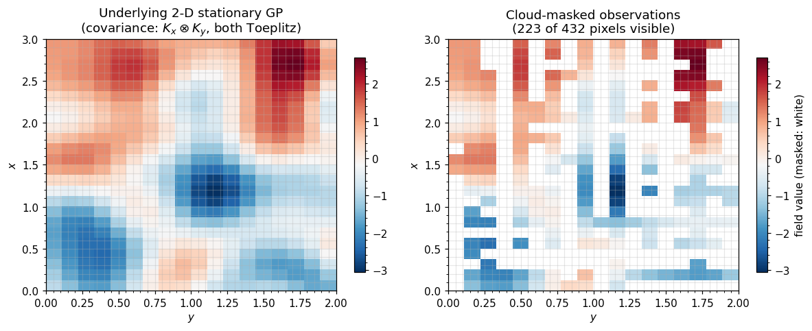

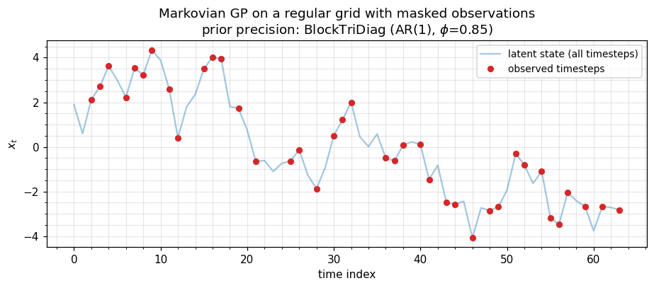
6. Markovian GPs — `MaskedOperator(BlockTriDiag, ...)`¶

State-space GPs (Matérn-1/2, -3/2, -5/2 in time; AR(p) priors; OU processes) have a BlockTriDiag precision on a regular time grid, with $O(Nd^3)$ Cholesky / solve / sampling. Real environmental timeseries arrive with gaps — GPS outages, sensor downtime, missed satellite passes, daily-vs-hourly scheduling. Masking lets us keep the cheap banded prior over the full timeline and select observed timesteps without ever forming a dense subset.

The pattern: build the state-space prior once on the regular grid, then MaskedOperator(prior, observation_mask, observation_mask) to obtain the prior covariance over observed timesteps for likelihood evaluation, conditional posterior, RTS smoothing, etc.

# AR(1)-as-state-space prior on a regular grid of N_t = 64 timesteps
N_t, d = 64, 1
phi, sigma2 = 0.85, 1.0
D_blocks = jnp.tile(((1.0 + phi**2) / sigma2) * jnp.eye(d), (N_t, 1, 1))
A_blocks = jnp.tile((-phi / sigma2) * jnp.eye(d), (N_t - 1, 1, 1))
D_blocks = D_blocks.at[0].set((1.0 / sigma2) * jnp.eye(d))
D_blocks = D_blocks.at[-1].set((1.0 / sigma2) * jnp.eye(d))
Lam = BlockTriDiag(D_blocks, A_blocks, tags=lx.positive_semidefinite_tag)

# Observation mask: 60% of timesteps observed, in clusters (geophysical-realistic)
keys = jax.random.split(jax.random.PRNGKey(60), 2)
obs_mask = jax.random.bernoulli(keys[0], p=0.6, shape=(N_t,))

# Masked Markov prior — keeps the full-grid banded prior intact, restricts I/O to observed times
M_markov = MaskedOperator(Lam, obs_mask, obs_mask, tags=lx.positive_semidefinite_tag)
print(f"full grid    : {N_t} timesteps")
print(f"observed     : {int(obs_mask.sum())} timesteps  ({100*float(obs_mask.mean()):.0f}%)")
print(f"masked shape : {M_markov.out_size()} x {M_markov.in_size()}")

# Sanity: matvec matches the explicit submatrix of the dense BTD precision
v = jax.random.normal(keys[1], (M_markov.in_size(),))
ref = Lam.as_matrix()[np.where(obs_mask)[0]][:, np.where(obs_mask)[0]] @ v
err = jnp.linalg.norm(M_markov.mv(v) - ref)
print(f"matvec error : {err:.2e}")

# Visualize: full timeline (one sample) + observation mask
L = cholesky(Lam)
z = jax.random.normal(jax.random.PRNGKey(61), (N_t * d,))
x_full = jax.scipy.linalg.solve_triangular(L.as_matrix().T, z, lower=False)
x_full = np.asarray(x_full)
t_grid = np.arange(N_t)

fig, ax = plt.subplots(figsize=(8.5, 3.8))
ax.plot(t_grid, x_full, "C0-", alpha=0.4, label="latent state (all timesteps)")
ax.plot(t_grid[np.asarray(obs_mask)], x_full[np.asarray(obs_mask)], "C3o", ms=5, label="observed timesteps")
ax.set_xlabel("time index"); ax.set_ylabel("$x_t$")
ax.set_title("Markovian GP on a regular grid with masked observations\n"
             rf"prior precision: BlockTriDiag (AR(1), $\phi$={phi})")
ax.legend(loc="upper right", fontsize=9)
plt.tight_layout()
plt.show()

full grid    : 64 timesteps
observed     : 39 timesteps  (61%)
masked shape : 39 x 39

matvec error : 1.67e-16

7. Asymmetric masking — cross-covariance for prediction¶

When you want $K_{*X}$ — covariance between test points (rows) and training points (columns) — pass different masks for rows and columns:

K_{*X} \;=\; \mathrm{MaskedOperator}(K, r=\text{test mask}, c=\text{train mask})

((4))

The result is rectangular and not square; matvec still costs the base operator’s price. This is the cheap path for posterior-mean prediction at held-out indices.

# Train / test split on the 1-D Toeplitz
np.random.seed(0)
all_idx = np.arange(n)
test_idx = np.random.choice(n, size=6, replace=False)
train_mask = jnp.array([i not in test_idx for i in all_idx])
test_mask  = jnp.array([i in test_idx for i in all_idx])
print(f"train : {int(train_mask.sum())} points")
print(f"test  : {int(test_mask.sum())} points")

K_starX = MaskedOperator(T, test_mask, train_mask)  # (test x train), no PSD tag (rectangular)

# Verify
ref_starX = T.as_matrix()[np.where(test_mask)[0]][:, np.where(train_mask)[0]]
v_train = jax.random.normal(jax.random.PRNGKey(30), (K_starX.in_size(),))
err = jnp.linalg.norm(K_starX.mv(v_train) - ref_starX @ v_train)
print(f"K_*X shape        : {K_starX.out_size()} x {K_starX.in_size()}")
print(f"K_*X matvec error : {err:.2e}")

train : 18 points
test  : 6 points

K_*X shape        : 6 x 18
K_*X matvec error : 2.00e-15

8. What masking does to the matrix — visualization gallery¶

The previous sections showed data under masking; this one shows the matrix. Each row pairs the full-grid base covariance (or precision) on the left with the masked sub-matrix on the right, so the action of the mask becomes legible:

Plain MVN: a generic dense Σ, with the masked rows/columns simply dropped.
Toeplitz: stationary kernel on a regular grid; masking destroys the constant-diagonal property, but the entries that survive are still pulled from the same kernel function.
BlockTriDiag (Markovian GP): banded precision; masked rows/columns punch holes through the bands.
Asymmetric / cross-covariance ( $K_{*X}$ ): rectangular, train rows × test columns — the predictive-mean primitive.

# Renumber the §-numbering inside the notebook is purely cosmetic — the existing
# operators (Sigma, T, Lam) are still in scope from the previous cells.
fig, axes = plt.subplots(4, 2, figsize=(10, 14))

# ----- Row 1: plain MVN base vs masked -----
mask_mvn = jnp.array([True]*4 + [False]*4 + [True]*4)
M_mvn = MaskedOperator(Sigma_op, mask_mvn, mask_mvn, tags=lx.positive_semidefinite_tag)
vmin, vmax = float(Sigma.min()), float(Sigma.max())
axes[0,0].imshow(Sigma, cmap="RdBu_r", vmin=vmin, vmax=vmax)
axes[0,0].set_title(rf"Plain MVN $\Sigma$  ({n_mvn}$\times${n_mvn})")
for k in jnp.where(~mask_mvn)[0]:
    axes[0,0].axhspan(int(k)-0.5, int(k)+0.5, color="grey", alpha=0.25)
    axes[0,0].axvspan(int(k)-0.5, int(k)+0.5, color="grey", alpha=0.25)
axes[0,1].imshow(M_mvn.as_matrix(), cmap="RdBu_r", vmin=vmin, vmax=vmax)
axes[0,1].set_title(rf"Masked $\Sigma_{{\rm obs}}$  ({M_mvn.out_size()}$\times${M_mvn.in_size()})  -- grey rows/cols dropped")

# ----- Row 2: Toeplitz base vs masked -----
T_dense = T.as_matrix()
mask_t = mask  # the §4 1-D mask, on the n=24 Toeplitz grid
M_t = MaskedOperator(T, mask_t, mask_t, tags=lx.positive_semidefinite_tag)
vmin_t, vmax_t = float(T_dense.min()), float(T_dense.max())
axes[1,0].imshow(T_dense, cmap="viridis", vmin=vmin_t, vmax=vmax_t)
axes[1,0].set_title(rf"Toeplitz base ($24\times 24$, RBF on regular grid)")
for k in jnp.where(~mask_t)[0]:
    axes[1,0].axhspan(int(k)-0.5, int(k)+0.5, color="white", alpha=0.4)
    axes[1,0].axvspan(int(k)-0.5, int(k)+0.5, color="white", alpha=0.4)
axes[1,1].imshow(M_t.as_matrix(), cmap="viridis", vmin=vmin_t, vmax=vmax_t)
axes[1,1].set_title(rf"Masked Toeplitz  ({M_t.out_size()}$\times${M_t.in_size()})  -- diagonals are no longer constant")

# ----- Row 3: Block-tridiagonal precision base vs masked -----
Lam_small_N, Lam_small_d = 12, 1
phi_s, sig2_s = 0.85, 1.0
D_s = jnp.tile(((1.0 + phi_s**2) / sig2_s) * jnp.eye(Lam_small_d), (Lam_small_N, 1, 1))
A_s = jnp.tile((-phi_s / sig2_s) * jnp.eye(Lam_small_d), (Lam_small_N - 1, 1, 1))
D_s = D_s.at[0].set((1.0 / sig2_s) * jnp.eye(Lam_small_d))
D_s = D_s.at[-1].set((1.0 / sig2_s) * jnp.eye(Lam_small_d))
Lam_s = BlockTriDiag(D_s, A_s, tags=lx.positive_semidefinite_tag)
mask_btd = jnp.array([True, True, False, True, True, True, False, False, True, True, True, True])
M_btd = MaskedOperator(Lam_s, mask_btd, mask_btd, tags=lx.positive_semidefinite_tag)
Lam_dense = Lam_s.as_matrix()
vmin_b, vmax_b = float(Lam_dense.min()), float(Lam_dense.max())
axes[2,0].imshow(Lam_dense, cmap="RdBu_r", vmin=vmin_b, vmax=vmax_b)
axes[2,0].set_title(r"BlockTriDiag precision $\Lambda$  ($12\times 12$, AR(1))")
for k in jnp.where(~mask_btd)[0]:
    axes[2,0].axhspan(int(k)-0.5, int(k)+0.5, color="grey", alpha=0.3)
    axes[2,0].axvspan(int(k)-0.5, int(k)+0.5, color="grey", alpha=0.3)
axes[2,1].imshow(M_btd.as_matrix(), cmap="RdBu_r", vmin=vmin_b, vmax=vmax_b)
axes[2,1].set_title(rf"Masked $\Lambda_{{\rm obs}}$  ({M_btd.out_size()}$\times${M_btd.in_size()})  -- bands punched through")

# ----- Row 4: Asymmetric / cross-covariance -----
# Reuse the §7 train/test split on the n=24 Toeplitz grid
axes[3,0].imshow(T_dense, cmap="viridis", vmin=vmin_t, vmax=vmax_t)
axes[3,0].set_title(r"Full Toeplitz $K$  -- highlight test rows + train cols")
for k in jnp.where(test_mask)[0]:
    axes[3,0].axhspan(int(k)-0.5, int(k)+0.5, color="C3", alpha=0.25)
for k in jnp.where(train_mask)[0]:
    axes[3,0].axvspan(int(k)-0.5, int(k)+0.5, color="C0", alpha=0.15)
axes[3,1].imshow(K_starX.as_matrix(), cmap="viridis", vmin=vmin_t, vmax=vmax_t, aspect="auto")
axes[3,1].set_title(rf"Cross-cov $K_{{*X}}$  ({K_starX.out_size()}$\times${K_starX.in_size()})  -- rectangular")

for ax in axes.flatten():
    ax.set_xticks([]); ax.set_yticks([])

plt.tight_layout()
plt.show()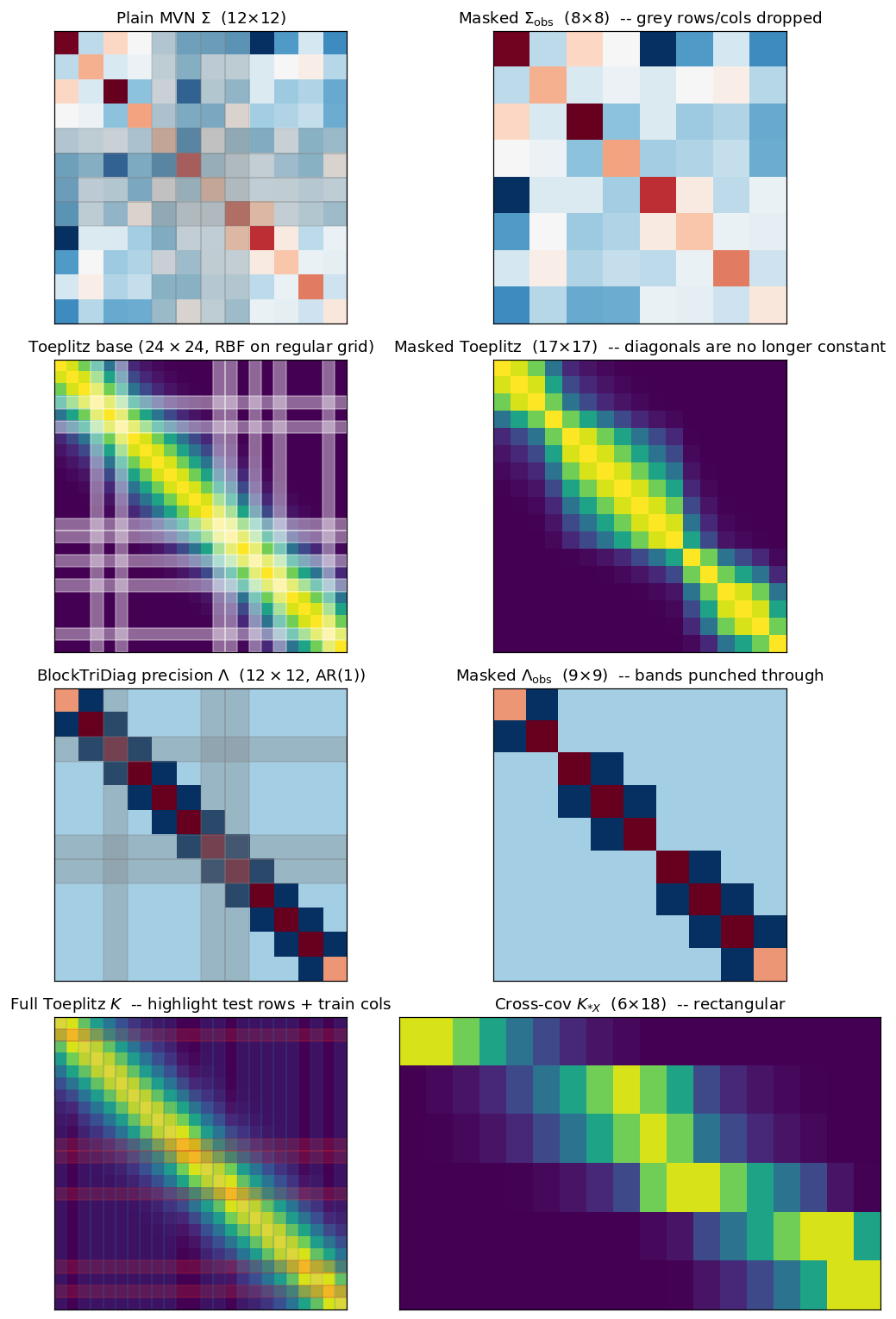

8. Solve and logdet — the catch¶

Masking destroys the structural identities that gave us cheap solve and logdet:

A masked Toeplitz is no longer Toeplitz (the masked rows/columns break the constant-diagonal property).
A masked Kronecker is no longer a Kronecker (the masked grid no longer factors as a tensor product).
A masked block-tridiagonal is still banded, with reshuffled bandwidth — sometimes useful, often not.

So solve(MaskedOperator(...)) and logdet(MaskedOperator(...)) typically fall back to either:

Dense materialization ( $\tilde A$ ) followed by Cholesky — $O(M^3)$ where $M$ is the observed count. Fine when $M$ is small.
Iterative Krylov (CG, MINRES, LSMR) using the structured matvec of the masked operator — $O(\text{iter} \cdot \text{base-mv-cost})$ per outer step. Fine when the base structure is preserved.

The right choice depends on the regime: mild missingness $M \approx N$ ⇒ iterative, heavy missingness $M \ll N$ ⇒ dense subset. The crossover for Toeplitz is roughly $M \sim N/\log N$ .

# Cost-table comparison (theoretical)
Ns = np.array([2**k for k in range(6, 18)])  # 64 .. 130k
M_frac = 0.7  # 30% missing
Ms = (M_frac * Ns).astype(int)

dense_full       = Ns**3 / 3
dense_subset     = Ms**3 / 3
masked_toeplitz_cg = 30 * Ms * np.log2(Ns)        # ~30 CG iterations × O(N log N) matvec
toeplitz_full_solve = Ns**2                       # Levinson-Durbin reference

fig, ax = plt.subplots(figsize=(7.5, 5.5))
ax.loglog(Ns, dense_full,           "C3-",  marker="o", label=r"dense full grid Cholesky")
ax.loglog(Ns, dense_subset,         "C0--", marker="s", label=rf"dense subset Cholesky ($M={int(M_frac*100)}\%N$)")
ax.loglog(Ns, masked_toeplitz_cg,   "C2-",  marker="^", label=r"masked-Toeplitz + CG ($30$ iter)")
ax.loglog(Ns, toeplitz_full_solve,  "C1:",  marker="D", label=r"full-grid Toeplitz Levinson")
ax.set_xlabel("full-grid size $N$")
ax.set_ylabel("FLOPs (theoretical)")
ax.set_title("Solve cost: dense subset vs masked-structured + CG")
ax.legend(loc="upper left")
plt.tight_layout()
plt.show()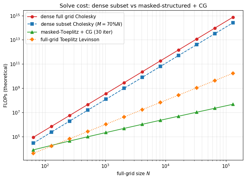

9. Summary — when to reach for `MaskedOperator`¶

A short cheat-sheet:

Scenario	Pattern
Subset of a generic MVN (CV folds, leave-one-out)	`MaskedOperator(MatrixLinearOperator(Σ), mask, mask)`
Markovian / state-space GP, missing timesteps (GPS, tide gauge, eddy-cov)	`MaskedOperator(BlockTriDiag, mask, mask)`
Stationary 1-D series, missing observations	`MaskedOperator(Toeplitz(c), mask, mask)`
2-D gridded field, cloud / valid mask	`MaskedOperator(Kronecker(T_x, T_y), m, m)`
Train→test cross-covariance	`MaskedOperator(K, test_mask, train_mask)` (asymmetric)
Heavy missingness ( $M \ll N$ )	materialize $\tilde A$ once, dense solve
Mild missingness ( $M \sim N$ )	masked-structured matvec inside CG / MINRES

Three notes:

MaskedOperator only carries PSD / symmetric tags when you pass them explicitly and only in the symmetric-masking case. Asymmetric masks produce rectangular operators and shouldn’t carry these tags.
For irregular timestamps with no underlying regular grid, MaskedOperator doesn’t apply — you fall back to dense covariance or inducing-point approximations (Part 5).
Combining with BlockTriDiag is what powers missing-data Kalman smoothing — masked observations + Markov prior, with all primitives staying $O(N)$ . We’ll revisit this pattern in Part 7 (state-space GPs).

The next notebook (1.7) wraps Part 1.A by explaining the structural-tag system that makes all of these dispatch decisions automatic — when gaussx.solve sees a BlockTriDiag tag, it routes to the banded sweep; when it sees a MaskedOperator wrapping a Kronecker, it knows to look at the base. Tags are how the operator catalog turns into a working dispatch system.