Conditioner architectures

02 — Conditioner architectures¶

This is the headline of Part 5. A coupling layer has two parts — the bijector $T$ (notebook 01) and the conditioner $c_\phi$ that reads the passive half and emits $T$ ’s parameters, $\theta = c_\phi(x_A)$ . The bijector is just a triangular wrapper that makes the log-det free; the conditioner is where the modelling power lives Papamakarios et al. (2021). Swap in a bigger or better-suited conditioner and the same coupling layer models far richer dependence — which is exactly why every structured-data part (images, sequences, graphs) revisits this menu and picks a modality-appropriate network.

In gauss_flows the conditioner is an equinox.nn.MLP sized by nn_width and nn_depth, reading $x_A$ and outputting all of the active half’s bijector parameters at once. We fix the bijector (mixture-CDF) and study the conditioner.

What you will see

The conditioner as the expressive engine: capacity (width) vs fit, the parameter-budget trade-off.
Output clamping (log_scale_bound): bounding the log-scale keeps training stable and lands a better optimum.
A map of the modality-specific conditioners that Parts 11–13 plug into this same slot.

import warnings

warnings.filterwarnings("ignore")

import equinox as eqx
import jax
import jax.numpy as jnp
import jax.random as jr
import matplotlib.pyplot as plt
import numpy as np
import optax
from flowjax.bijections import Chain, Flip, Invert
from flowjax.distributions import Normal, Transformed

import gauss_flows as gf
from gauss_flows._src.transforms.bijections.linear.rotation import HouseholderRotation
from _style import SCATTER_KW, style_ax

jax.config.update("jax_enable_x64", True)

# Spiral target (needs cross-coordinate structure -> stresses the conditioner).
rng = np.random.default_rng(0)
n = 3000
t = rng.uniform(0.5, 3.5, n)
arm = (rng.integers(0, 2, n) * 2 - 1)[:, None]
xy = arm * np.stack([t * np.cos(2.5 * t), t * np.sin(2.5 * t)], axis=1) + 0.08 * rng.standard_normal((n, 2))
X = jnp.asarray((xy - xy.mean(0)) / xy.std(0))


def build(key, *, n_blocks=3, width=32, depth=2, log_scale_bound=5.0):
    """Stack of mixture-CDF coupling blocks with a configurable MLP conditioner."""
    bijections = []
    for k in jr.split(key, n_blocks):
        rk, c1, c2 = jr.split(k, 3)
        rot = HouseholderRotation(n_reflections=2, shape=(2,))
        rot = eqx.tree_at(lambda r: r.params, rot, jr.normal(rk, rot.params.shape))
        mk = lambda kk: gf.MixtureGaussianCDFCoupling(
            kk, shape=(2,), n_components=8, nn_width=width, nn_depth=depth,
            log_scale_bound=log_scale_bound)
        bijections += [rot, mk(c1), Flip(shape=(2,)), mk(c2), Flip(shape=(2,))]
    return Transformed(Normal(jnp.zeros(2)), Invert(Chain(bijections)))


def train(flow, *, steps=1200, peak_lr=3e-3, batch=512, seed=1, track=False):
    params, static = eqx.partition(flow, eqx.is_inexact_array)
    schedule = optax.cosine_onecycle_schedule(steps, peak_lr)
    opt = optax.chain(optax.clip_by_global_norm(1.0), optax.adam(schedule))
    state = opt.init(params)

    @eqx.filter_jit
    def step(params, state, xb):
        loss, g = eqx.filter_value_and_grad(
            lambda p: -jnp.mean(jax.vmap(eqx.combine(p, static).log_prob)(xb)))(params)
        upd, state = opt.update(g, state)
        return eqx.apply_updates(params, upd), state, loss

    key, traj = jr.key(seed), []
    for i in range(steps):
        key, sk = jr.split(key)
        params, state, loss = step(params, state, X[jr.randint(sk, (batch,), 0, X.shape[0])])
        if track and i % 25 == 0:
            traj.append(float(loss))
    return eqx.combine(params, static), np.array(traj)


n_params = lambda f: int(sum(x.size for x in jax.tree_util.tree_leaves(eqx.filter(f, eqx.is_inexact_array))))
logp = lambda f: float(jax.vmap(f.log_prob)(X).mean())

1. The conditioner is the expressive engine¶

Inside each coupling, the conditioner is a plain MLP: input dimension $= |A|$ (the passive half), output dimension $=$ the number of bijector parameters for the active half. Everything the layer can model — how the transform of $x_B$ bends with $x_A$ — is what this network can represent. We inspect one.

probe = gf.MixtureGaussianCDFCoupling(jr.key(0), shape=(2,), n_components=8,
                                      nn_width=32, nn_depth=2)
mlp = probe._coupling.conditioner
print(f"conditioner is an {type(mlp).__name__} with {len(mlp.layers)} Linear layers:")
for layer in mlp.layers:
    print(f"  Linear: in={layer.weight.shape[1]:3d} -> out={layer.weight.shape[0]:3d}")
print("  (input = passive coords; output = all bijector params for the active half)")

conditioner is an MLP with 3 Linear layers:
  Linear: in=  1 -> out= 32
  Linear: in= 32 -> out= 32
  Linear: in= 32 -> out= 24
  (input = passive coords; output = all bijector params for the active half)

A 1→32→32→24 MLP: it reads one passive coordinate and emits the 24 mixture-CDF parameters that define the active coordinate’s transform. The bijector form is fixed; the conditioner decides how expressively the transform reacts to context. So capacity should track the conditioner’s size.

2. Parameter budget vs expressiveness¶

We fix the bijector and the depth, sweep the conditioner width, and fit the spiral. Wider conditioners model more, with diminishing returns — the classic capacity curve.

widths = [4, 8, 16, 32, 64]
sweep = {w: train(build(jr.key(0), width=w))[0] for w in widths}
pts = [(n_params(sweep[w]), logp(sweep[w])) for w in widths]
for w, (p, lp) in zip(widths, pts):
    print(f"  nn_width={w:3d}: {p:6d} params -> log p {lp:.3f}")

fig, ax = plt.subplots(figsize=(7.4, 4.4))
ax.plot([p for p, _ in pts], [lp for _, lp in pts], "o-", color="tab:green", lw=2, ms=7)
for w, (p, lp) in zip(widths, pts):
    ax.annotate(f"w={w}", (p, lp), textcoords="offset points", xytext=(6, -10), fontsize=8)
ax.set(title="Conditioner capacity vs fit (bijector fixed)",
       xlabel="conditioner parameters (log scale)", ylabel="mean log p(x)", xscale="log")
style_ax(ax)
fig.tight_layout()

  nn_width=  4:    904 params -> log p -2.037
  nn_width=  8:   1840 params -> log p -1.918
  nn_width= 16:   4288 params -> log p -1.713
  nn_width= 32:  11488 params -> log p -1.686
  nn_width= 64:  35104 params -> log p -1.400

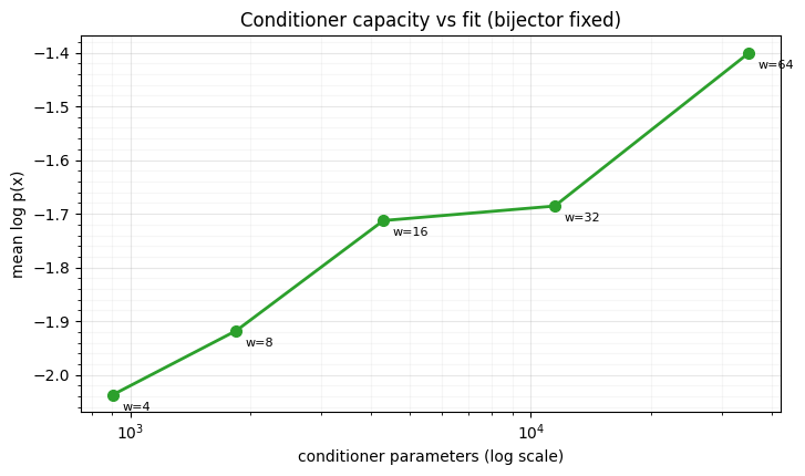
Likelihood climbs steadily with conditioner width — same bijector, same depth, the only thing growing is the network that reads context. The gains taper in the middle and pick up again with a much wider net: capacity is real but not free, the trade-off the master list calls parameter budget vs expressiveness. (Depth is the other knob; a shared-MLP conditioner — one trunk with per-coordinate heads — is the parameter-efficient variant when the active half is high-dimensional.)

3. Output clamping for stability¶

The conditioner outputs include log-scales. Left unbounded, a single bad batch can push a log-scale large, the coupling momentarily explodes or collapses volume, and training spikes. MixtureGaussianCDFCoupling’s log_scale_bound clamps the log-scale to $[-b, b]$ (via a smooth squash), a standard stabiliser. We train with a tight bound and a loose one and watch the loss.

tight, traj_tight = train(build(jr.key(0), log_scale_bound=3.0), track=True)
loose, traj_loose = train(build(jr.key(0), log_scale_bound=50.0), track=True)
print(f"tight clamp (b=3) : final log p {logp(tight):.3f}, peak training loss {traj_tight.max():.1f}")
print(f"loose clamp (b=50): final log p {logp(loose):.3f}, peak training loss {traj_loose.max():.1f}")

fig, ax = plt.subplots(figsize=(7.6, 4.4))
ax.plot(np.arange(len(traj_tight)) * 25, traj_tight, color="tab:green", lw=2, label="log_scale_bound = 3 (tight)")
ax.plot(np.arange(len(traj_loose)) * 25, traj_loose, color="tab:red", lw=2, alpha=0.8, label="log_scale_bound = 50 (loose)")
ax.set(title="Clamping the log-scale stabilises training",
       xlabel="step", ylabel="NLL (training batch)", ylim=(1, 8))
ax.legend(fontsize=9); style_ax(ax)
fig.tight_layout()

tight clamp (b=3) : final log p -1.628, peak training loss 3.5
loose clamp (b=50): final log p -1.906, peak training loss 17.8

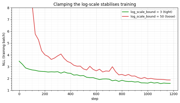
The tight clamp trains smoothly to a better optimum; the loose one spikes (its log-scale wanders far enough to momentarily wreck the likelihood) and settles higher. Even with gradient clipping in the optimiser, bounding the parameterised log-scale is a cheap, effective second line of defence — and the reason coupling layers expose log_scale_bound.

Everything above used an MLP because the data is an unstructured 2-D vector. The coupling contract does not care what $c_\phi$ is, so the conditioner is the natural place to inject domain structure:

data	conditioner	where
vectors	MLP / shared-MLP / ResNet	here (5.C)
images	CNN (preserves spatial dims)	Part 12
sequences	RNN / Transformer / Mamba (causal)	Part 11
graphs	message-passing GNN	Part 5 (research)
symmetric domains	equivariant network	Parts 12–13

Same triangular-Jacobian, free-log-det coupling; only the network reading $x_A$ changes. That modularity is why coupling flows generalise across modalities.

Recap¶

knob	effect
conditioner width / depth	capacity → expressiveness (diminishing returns)
shared-MLP trunk + heads	parameter-efficient for high-dim active halves
`log_scale_bound`	clamps log-scale → stable training, better optimum
conditioner architecture	injects modality structure (CNN / RNN / GNN / equivariant)

The bijector sets what shape a coordinate map can take; the conditioner sets how richly it reacts to the rest of the data — and it is the part you swap per domain.

Next up. A coupling layer only transforms half the coordinates, so which half, and how the halves alternate, matters. 03 — Mask design covers checkerboard / channel-wise / learned masks and how stacking them gives every coordinate both roles.

References¶

Papamakarios, G., Nalisnick, E., Rezende, D. J., Mohamed, S., & Lakshminarayanan, B. (2021). Normalizing Flows for Probabilistic Modeling and Inference. Journal of Machine Learning Research, 22(57), 1–64.

02 — Conditioner architectures¶

1. The conditioner is the expressive engine¶

2. Parameter budget vs expressiveness¶

3. Output clamping for stability¶

4. The conditioner menu — where Parts 11–13 plug in¶

Recap¶