Mask design for coupling flows

03 — Mask design for coupling flows¶

The coupling contract (notebook 00) has a catch: a coupling layer transforms only the active half and copies the passive half through unchanged. A single layer is therefore not a bijector that can reshape every coordinate — and if every layer uses the same split, the passive coordinates are never touched, no matter how deep the stack. The mask decides the split, and alternating it is what makes a coupling flow a full transform: each coordinate must be transformed in some layers and serve as context in others.

What you will see

The failure: a stack with a fixed mask leaves half the coordinates exactly at their input values.
The fix: alternating the mask (a Flip between layers) Gaussianizes every coordinate and fits better.
The mask families — channel-wise, checkerboard, learned — and why images use a different pattern than vectors.

import warnings

warnings.filterwarnings("ignore")

import equinox as eqx
import jax
import jax.numpy as jnp
import jax.random as jr
import matplotlib.pyplot as plt
import numpy as np
import optax
from flowjax.bijections import Chain, Flip, Invert
from flowjax.distributions import Normal, Transformed

import gauss_flows as gf
from _style import GAUSS_KW, SCATTER_KW, standard_normal_pdf, style_ax

jax.config.update("jax_enable_x64", True)

from sklearn.datasets import make_moons
X_np, _ = make_moons(n_samples=3000, noise=0.07, random_state=0)
X = jnp.asarray((X_np - X_np.mean(0)) / X_np.std(0))


def coupling(key):
    return gf.MixtureGaussianCDFCoupling(key, shape=(2,), n_components=8, nn_width=32, nn_depth=2)


def stack(key, n_blocks, *, alternate):
    """Stack of couplings; with `alternate`, a Flip between layers swaps the mask."""
    bijections = []
    for k in jr.split(key, n_blocks):
        bijections.append(coupling(k))
        if alternate:
            bijections.append(Flip(shape=(2,)))
    return Transformed(Normal(jnp.zeros(2)), Invert(Chain(bijections)))


to_latent = lambda flow: np.asarray(jax.vmap(flow.bijection.inverse)(X))   # data -> z

1. A fixed mask leaves half the coordinates untouched¶

gf couplings split into a fixed passive/active half. A single layer leaves coord 0 exactly as it came in; stacking more of the same layer changes nothing about coord 0. We build a 4-block fixed-mask stack and check the latent.

single = coupling(jr.key(0))
delta = np.asarray(single.transform(jnp.array([0.5, 0.5])) - jnp.array([0.5, 0.5]))
print(f"single coupling: change per coord = {np.round(delta, 4)}  -> coord 0 is passive")

fixed = stack(jr.key(0), 4, alternate=False)
z_fixed = to_latent(fixed)
print(f"\n4-block FIXED-mask stack:")
print(f"  latent coord 0 identical to input? {np.allclose(z_fixed[:, 0], np.asarray(X[:, 0]), atol=1e-6)}")
print(f"  latent coord 0 std = {z_fixed[:, 0].std():.3f}  (input was standardised; not Gaussianized)")

single coupling: change per coord = [ 0.     -0.1723]  -> coord 0 is passive


4-block FIXED-mask stack:
  latent coord 0 identical to input? True
  latent coord 0 std = 1.000  (input was standardised; not Gaussianized)

The passive coordinate comes out bit-for-bit unchanged — four layers did nothing to it, because every layer used the same mask. So its latent marginal is still the (non-Gaussian) data marginal, not $\mathcal{N}(0,1)$ . The flow has no way to Gaussianize half its inputs.

2. Alternating the mask fixes it¶

Insert a Flip between layers and the roles swap: coord 0 is passive in one layer, active in the next. Now every coordinate is both transformed and used as context. We compare the latent marginals.

alt = stack(jr.key(0), 4, alternate=True)
z_alt = to_latent(alt)

zz = np.linspace(-3.5, 3.5, 200)
fig, axes = plt.subplots(1, 2, figsize=(11, 4.2), sharey=True)
for ax, zc, title in [(axes[0], z_fixed, "fixed mask"), (axes[1], z_alt, "alternating mask")]:
    ax.hist(zc[:, 0], bins=60, density=True, alpha=0.7, color="tab:red" if title == "fixed mask" else "tab:green",
            label="latent coord 0")
    ax.plot(zz, standard_normal_pdf(zz), **GAUSS_KW, label=r"$\mathcal{N}(0,1)$")
    ax.set(title=f"{title}: coord-0 latent  (std {zc[:, 0].std():.2f})", xlabel="$z_0$")
    ax.legend(fontsize=8); style_ax(ax)
axes[0].set_ylabel("density")
fig.suptitle("Fixed mask never Gaussianizes coord 0; alternating does", y=1.02)
fig.tight_layout()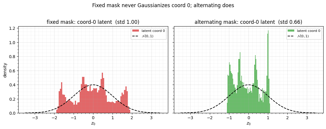

With a fixed mask the coord-0 latent is the untouched (flat, non-Gaussian) data marginal; alternating the mask pulls it toward $\mathcal{N}(0,1)$ . The likelihood follows — we fit both.

def train(flow, *, steps=1200, peak_lr=3e-3, batch=512, seed=1):
    params, static = eqx.partition(flow, eqx.is_inexact_array)
    schedule = optax.cosine_onecycle_schedule(steps, peak_lr)
    opt = optax.chain(optax.clip_by_global_norm(1.0), optax.adam(schedule))
    state = opt.init(params)

    @eqx.filter_jit
    def step(params, state, xb):
        loss, g = eqx.filter_value_and_grad(
            lambda p: -jnp.mean(jax.vmap(eqx.combine(p, static).log_prob)(xb)))(params)
        upd, state = opt.update(g, state)
        return eqx.apply_updates(params, upd), state, loss

    key = jr.key(seed)
    for _ in range(steps):
        key, sk = jr.split(key)
        params, state, _ = step(params, state, X[jr.randint(sk, (batch,), 0, X.shape[0])])
    return eqx.combine(params, static)


logp = lambda f: float(jax.vmap(f.log_prob)(X).mean())
print(f"fit (two-moons):  fixed mask = {logp(train(fixed)):.3f}   "
      f"alternating = {logp(train(alt)):.3f}")

fit (two-moons):  fixed mask = -1.685   alternating = -1.469

The alternating stack fits clearly better — and would Gaussianize both axes, which the fixed stack structurally cannot. Alternation is not optional; it is what turns a half-transform into a full one.

3. The mask families¶

Which split to use depends on the data’s structure. For an unstructured vector the channel-wise split (first half vs second half, alternated by Flip) is standard. For an image, neighbouring pixels are highly correlated, so a checkerboard mask keeps each transformed pixel surrounded by context pixels; channel-wise masks then split feature channels at coarser scales. Learned masks (a differentiable Gumbel-softmax over the split) are an option when the right partition is not obvious.

fig, axes = plt.subplots(1, 3, figsize=(13, 4.0))
# channel-wise (vector): first half passive, second active, then flipped
cw = np.zeros((1, 8)); cw[0, 4:] = 1
axes[0].imshow(np.repeat(cw, 2, axis=0), cmap="coolwarm", vmin=0, vmax=1, aspect="auto")
axes[0].set(title="channel-wise (vector)\npassive | active", xticks=range(8), yticks=[])
# checkerboard (image)
g = np.indices((8, 8)).sum(0) % 2
axes[1].imshow(g, cmap="coolwarm", vmin=0, vmax=1)
axes[1].set(title="checkerboard (image)\nactive pixels see neighbours", xticks=[], yticks=[])
# alternation across layers (channel-wise + flip)
layers = np.array([[0, 0, 1, 1], [1, 1, 0, 0], [0, 0, 1, 1]])
axes[2].imshow(layers, cmap="coolwarm", vmin=0, vmax=1, aspect="auto")
axes[2].set(title="stacking: alternate each layer\n(every coord gets both roles)",
            xlabel="coordinate", ylabel="layer", xticks=range(4), yticks=range(3))
for ax in (axes[0], axes[1]):
    ax.grid(False)
fig.suptitle("Mask families: blue = passive (context), red = active (transformed)", y=1.03)
fig.tight_layout()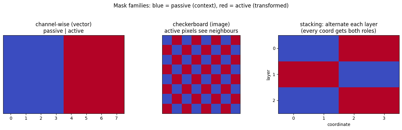

All three panels encode the same idea: blue coordinates are copied and used as context, red coordinates are transformed. The checkerboard’s value is locality — every active pixel is conditioned on its immediate neighbours — which is why image flows (Part 12) alternate checkerboard and channel-wise masks across scales. For our 2-D vectors, channel-wise + Flip is the whole story.

Recap¶

mask	data	role
channel-wise (split halves)	vectors / feature channels	standard RealNVP split
checkerboard	images	active pixels conditioned on neighbours
learned (Gumbel-softmax)	when partition is unclear	differentiable split
alternation across layers	all	gives every coordinate both roles — required

A coupling layer is half a transform; the mask schedule is what assembles halves into a full, every-coordinate bijector. Get it wrong (fixed mask) and a chunk of your data is never modelled.

Next up. With the coupling pattern, bijector menu, conditioners, and masks in hand, we can ask the comparative questions. 04 — Diagonal vs coupling (parameter-fair) and 05 — RBIG warm-start for coupling (the zero-kernel contract) revisit coupling against the diagonal flows of Part 4, leading into the formal coupling↔diagonal equivalence.