The bijector menu for coupling

01 — The bijector menu for coupling¶

Notebook 00 showed the coupling contract — triangular Jacobian, free log-det, analytic inverse — holds for any elementwise monotone bijector $T$ . The bijector and the conditioner are independent choices: this notebook fixes the conditioner (a small MLP) and tours the $T$ menu that gauss_flows offers. The choice sets how much each coupling layer can bend a coordinate.

bijector	$T(x_B)$	inverse	lineage
affine	$s\,x_B + t$	closed form	RealNVP Dinh et al. (2017)
mixture-CDF	$\Phi^{-1}\!\big(\sum_k\pi_k\Phi(x_B;\mu_k,\sigma_k)\big)$	root-find	Part 1 01
deep-sigmoid	cascaded σ-shifts	root-find	NAF-style
RQ-spline	piecewise rational-quadratic	closed form	NSF Durkan et al. (2019)

What you will see

Each bijector as a 1-D map of the active coordinate — affine is a straight line, the rest are monotone curves.
The family of maps the conditioner can dial: affine can only pick a line; expressive bijectors pick arbitrary monotone shapes.
An expressiveness comparison on a spiral: the spline and mixture-CDF fit best.

import warnings

warnings.filterwarnings("ignore")

import equinox as eqx
import jax
import jax.numpy as jnp
import jax.random as jr
import matplotlib.pyplot as plt
import numpy as np
import optax
from flowjax.bijections import Chain, Flip, Invert
from flowjax.distributions import Normal, Transformed

import gauss_flows as gf
from gauss_flows._src.transforms.bijections.linear.rotation import HouseholderRotation
from _style import GAUSS_KW, SCATTER_KW, style_ax

jax.config.update("jax_enable_x64", True)

# Builders for each coupling bijector, with a shared small MLP conditioner.
COUPLINGS = {
    "affine": (gf.AffineCoupling, {}),
    "mixture-CDF": (gf.MixtureGaussianCDFCoupling, {"n_components": 8}),
    "deep-sigmoid": (gf.DeepSigmoidCoupling, {"n_components": 8}),
    "RQ-spline": (gf.RQSplineCoupling, {"n_bins": 8, "interval": 4.0}),
}
COLORS = {"affine": "tab:red", "mixture-CDF": "tab:blue",
          "deep-sigmoid": "tab:purple", "RQ-spline": "tab:green"}


def make_coupling(name, key):
    cls, kw = COUPLINGS[name]
    return cls(key, shape=(2,), nn_width=32, nn_depth=2, **kw)

1. Each bijector is a per-coordinate monotone map¶

In a 2-D coupling the active coordinate $x_1$ is transformed conditioned on the passive $x_0$ . Fix $x_0$ and sweep $x_1$ : the bijector traces a 1-D monotone map $x_1 \mapsto z_1$ . Its shape is the bijector’s expressiveness.

xb = np.linspace(-3, 3, 200)
x0 = 0.7
fig, ax = plt.subplots(figsize=(6.4, 5.0))
ax.plot([-3, 3], [-3, 3], **GAUSS_KW, label="identity")
print("nonlinearity (max deviation from a straight line):")
for name in COUPLINGS:
    b = make_coupling(name, jr.key(3))
    zb = np.array([float(b.transform(jnp.array([x0, x]))[1]) for x in xb])
    p = np.polyfit(xb, zb, 1)
    nonlin = float(np.abs(zb - np.polyval(p, xb)).max())
    print(f"  {name:13s}: {nonlin:.3f}")
    ax.plot(xb, zb, color=COLORS[name], lw=2, label=f"{name}")
ax.set(title="The bijector as a 1-D map ($x_0$ fixed)\naffine is a line; the rest bend",
       xlabel="active input $x_1$", ylabel="output $z_1 = T(x_1)$", ylim=(-4, 4))
ax.legend(fontsize=8); style_ax(ax)
fig.tight_layout()

nonlinearity (max deviation from a straight line):

  affine       : 0.000

  mixture-CDF  : 0.258

  deep-sigmoid : 0.750

  RQ-spline    : 0.151

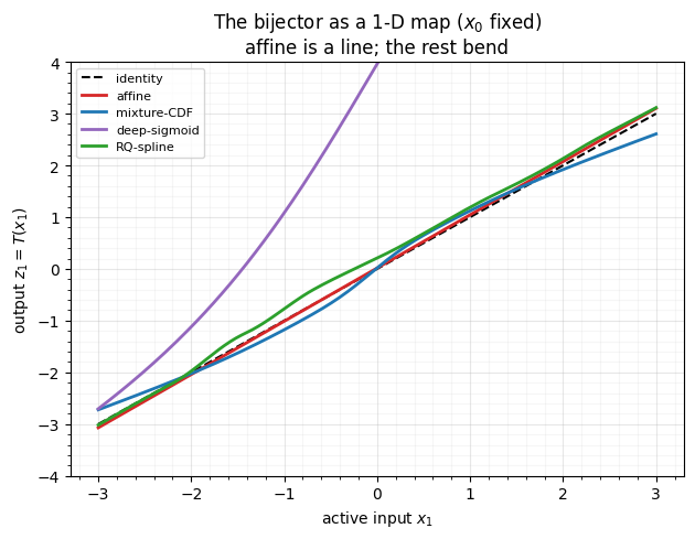
Affine is a straight line — a coupling layer with an affine $T$ can only scale and shift a coordinate (nonlinearity $\approx 0$ ). The mixture-CDF and rational-quadratic spline bend into smooth monotone S-curves; the deep-sigmoid bends most aggressively (and can get steep). All stay monotone — they must, to be invertible.

2. Expressiveness is the family of maps the conditioner can dial¶

The conditioner reads $x_0$ and emits $T$ ’s parameters, so as $x_0$ varies the layer sweeps a whole family of 1-D maps. That family is the layer’s true capacity. For affine the family is all lines (the conditioner only picks slope and intercept); for the spline it is a family of arbitrary monotone curves.

fig, axes = plt.subplots(1, 2, figsize=(11, 4.6), sharex=True, sharey=True)
for ax, name in zip(axes, ["affine", "RQ-spline"]):
    b = make_coupling(name, jr.key(3))
    for x0v in np.linspace(-2, 2, 7):
        zb = np.array([float(b.transform(jnp.array([x0v, x]))[1]) for x in xb])
        ax.plot(xb, zb, color=COLORS[name], lw=1.5, alpha=0.55)
    ax.plot([-3, 3], [-3, 3], **GAUSS_KW)
    ax.set(title=f"{name}: family over $x_0\\in[-2,2]$", xlabel="$x_1$", ylim=(-4, 4))
    style_ax(ax)
axes[0].set_ylabel("$z_1 = T_{\\theta(x_0)}(x_1)$")
fig.suptitle("What the conditioner can dial: lines (affine) vs curves (spline)", y=1.02)
fig.tight_layout()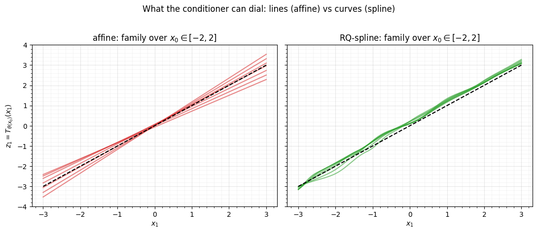

The affine panel is a sheaf of straight lines — every coordinate map the layer can produce is linear, so non-linear dependence must be built up across many stacked layers. The spline panel is a sheaf of distinct curves: a single layer can model a non-linear, context-dependent transform. That is why expressive bijectors need fewer layers.

3. Expressiveness in practice¶

We make this concrete: fit a small flow (2 coupling blocks) with each bijector on a spiral and compare held-out log-likelihood. With so few blocks, the per-bijector expressiveness — not depth — decides the fit.

rng = np.random.default_rng(0)
n = 3000
t = rng.uniform(0.5, 3.5, n)
arm = (rng.integers(0, 2, n) * 2 - 1)[:, None]
xy = arm * np.stack([t * np.cos(2.5 * t), t * np.sin(2.5 * t)], axis=1) + 0.08 * rng.standard_normal((n, 2))
X = jnp.asarray((xy - xy.mean(0)) / xy.std(0))


def build_flow(name, key, n_blocks=2):
    bijections = []
    for k in jr.split(key, n_blocks):
        rk, c1, c2 = jr.split(k, 3)
        rot = HouseholderRotation(n_reflections=2, shape=(2,))
        rot = eqx.tree_at(lambda r: r.params, rot, jr.normal(rk, rot.params.shape))
        bijections += [rot, make_coupling(name, c1), Flip(shape=(2,)),
                       make_coupling(name, c2), Flip(shape=(2,))]
    return Transformed(Normal(jnp.zeros(2)), Invert(Chain(bijections)))


def train(flow, steps=1500, peak_lr=3e-3, batch=512, seed=1):
    params, static = eqx.partition(flow, eqx.is_inexact_array)
    schedule = optax.cosine_onecycle_schedule(steps, peak_lr)
    opt = optax.chain(optax.clip_by_global_norm(1.0), optax.adam(schedule))
    state = opt.init(params)

    @eqx.filter_jit
    def step(params, state, xb):
        loss, g = eqx.filter_value_and_grad(
            lambda p: -jnp.mean(jax.vmap(eqx.combine(p, static).log_prob)(xb)))(params)
        upd, state = opt.update(g, state)
        return eqx.apply_updates(params, upd), state, loss

    key = jr.key(seed)
    for _ in range(steps):
        key, sk = jr.split(key)
        params, state, _ = step(params, state, X[jr.randint(sk, (batch,), 0, X.shape[0])])
    return eqx.combine(params, static)


logp = lambda f: float(jax.vmap(f.log_prob)(X).mean())
fitted = {name: train(build_flow(name, jr.key(0))) for name in COUPLINGS}
for name, f in fitted.items():
    print(f"{name:13s}: log p = {logp(f):.3f}")

fig, ax = plt.subplots(figsize=(7.0, 4.3))
names = list(COUPLINGS)
ax.bar(names, [logp(fitted[n]) for n in names], color=[COLORS[n] for n in names])
ax.set(title="Spiral fit with 2 coupling blocks (higher = better)",
       ylabel="mean log p(x)")
ax.tick_params(axis="x", labelrotation=15); style_ax(ax)
fig.tight_layout()

affine       : log p = -2.177

mixture-CDF  : log p = -1.564

deep-sigmoid : log p = -2.421

RQ-spline    : log p = -1.471

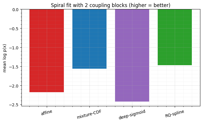
The rational-quadratic spline and mixture-CDF fit the spiral best — their expressive per-coordinate curves capture the bend in just two blocks. Affine lags: linear per-coordinate maps need more depth to compose the same shape. Deep-sigmoid is expressive in principle (its 1-D map bent the most in §1) but its steep, unbounded maps make it the hardest to optimise here — a reminder that raw flexibility is not the same as trainability. We compare the weakest and strongest densities.

gx, gy = np.meshgrid(np.linspace(-2.5, 2.5, 120), np.linspace(-2.5, 2.5, 120))
grid = jnp.asarray(np.column_stack([gx.ravel(), gy.ravel()]))
fig, axes = plt.subplots(1, 3, figsize=(14.5, 4.6))
axes[0].scatter(X[:, 0], X[:, 1], color="tab:blue", **SCATTER_KW)
axes[0].set(title="data (spiral)", xlabel="$x_0$", ylabel="$x_1$")
for ax, name in zip(axes[1:], ["affine", "RQ-spline"]):
    lp = np.asarray(jax.vmap(fitted[name].log_prob)(grid)).reshape(gx.shape)
    ax.contourf(gx, gy, np.exp(lp), levels=18, cmap="viridis")
    ax.scatter(X[:, 0], X[:, 1], s=3, color="white", alpha=0.2)
    ax.set(title=f"{name} (2 blocks)\nlog p = {logp(fitted[name]):.2f}", xlabel="$x_0$")
for ax in axes:
    ax.set_aspect("equal"); style_ax(ax)
fig.suptitle("Affine vs RQ-spline at equal depth", y=1.02)
fig.tight_layout()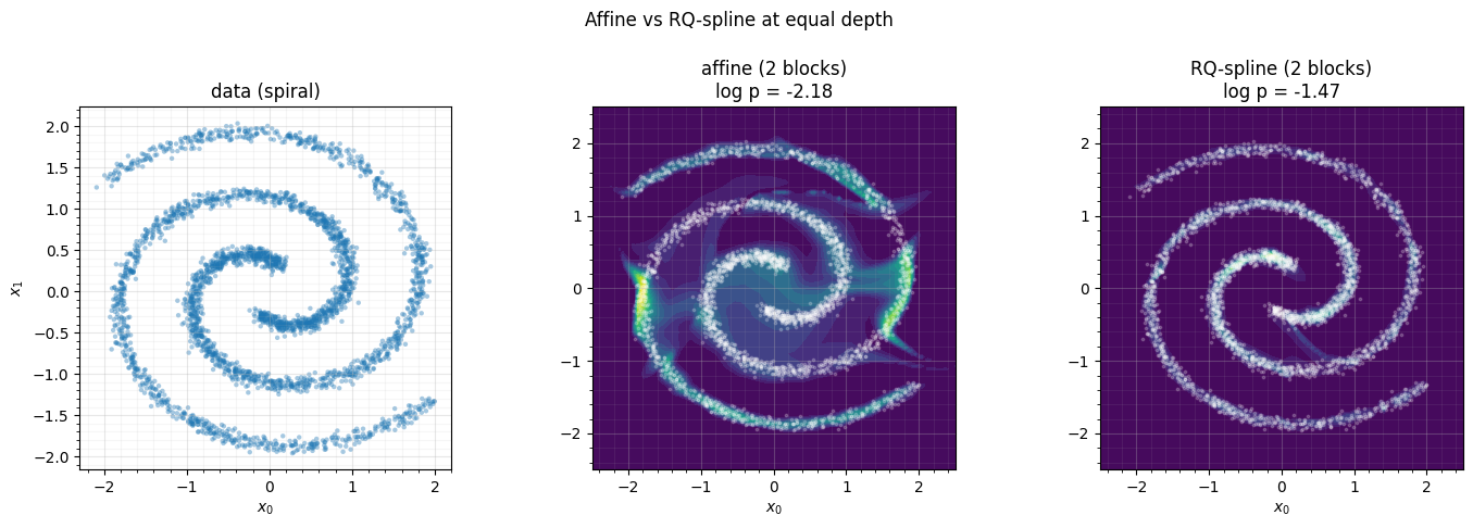

Recap¶

bijector	per-coordinate map	inverse	notes
affine	linear ( $s\,x+t$ )	closed form	cheapest; RealNVP; needs depth for non-linearity
mixture-CDF	smooth monotone S	root-find	reuses Part 1’s marginal; analytic log-det
deep-sigmoid	cascaded σ	root-find	very flexible, but steep & harder to train
RQ-spline	piecewise rational-quadratic	closed form	NSF; expressive and exactly invertible — the modern default

The bijector sets per-layer expressiveness; the spline’s closed-form inverse and analytic log-det (Part 1 02) make it the usual choice. But the other half of a coupling layer — the conditioner — is where most of the modelling power lives.

Next up. 02 — Conditioner architectures: the network that reads $x_A$ and emits θ is the expressive engine; we tour MLP / shared-MLP / ResNet conditioners, output clamping for stability, and the parameter-budget-vs-expressiveness trade-off.

References¶

Dinh, L., Sohl-Dickstein, J., & Bengio, S. (2017). Density Estimation using Real NVP. International Conference on Learning Representations (ICLR).
Durkan, C., Bekasov, A., Murray, I., & Papamakarios, G. (2019). Neural Spline Flows. Advances in Neural Information Processing Systems (NeurIPS).