Depth, residual coupling & stability

07 — Depth, residual coupling & stability¶

We have the pieces of a coupling layer — the pattern, the bijector, the conditioner, the mask. A single layer transforms only half the coordinates, so a coupling flow’s power comes from stacking: $T = T_L \circ \cdots \circ T_1$ with alternating masks (notebook 03), each block adding expressiveness. This notebook looks at the depth dimension — how much it buys, what keeps deep stacks trainable, and the residual coupling variant that points ahead to Part 9.

What you will see

Depth → expressiveness: stacking coupling blocks steadily improves the fit.
Stability: gradient clipping keeps a deep stack training well; a note on ActNorm pre-conditioning and the warm-start.
Residual coupling ( $T(x) = x + g(x)$ ): why invertibility needs $\mathrm{Lip}(g)<1$ and the inverse is a Banach fixed-point iteration — a preview of implicit flows.

import warnings

warnings.filterwarnings("ignore")

import equinox as eqx
import jax
import jax.numpy as jnp
import jax.random as jr
import matplotlib.pyplot as plt
import numpy as np
import optax
from flowjax.bijections import Chain, Flip, Invert
from flowjax.distributions import Normal, Transformed

import gauss_flows as gf
from gauss_flows._src.transforms.bijections.linear.rotation import HouseholderRotation
from _style import GAUSS_KW, style_ax

jax.config.update("jax_enable_x64", True)

rng = np.random.default_rng(0)
n = 3000
t = rng.uniform(0.5, 3.5, n)
arm = (rng.integers(0, 2, n) * 2 - 1)[:, None]
xy = arm * np.stack([t * np.cos(2.5 * t), t * np.sin(2.5 * t)], axis=1) + 0.08 * rng.standard_normal((n, 2))
X = jnp.asarray((xy - xy.mean(0)) / xy.std(0))


def build(key, depth, *, coupling="spline", actnorm=False):
    bijections = []
    for k in jr.split(key, depth):
        rk, c1, c2 = jr.split(k, 3)
        rot = HouseholderRotation(n_reflections=2, shape=(2,))
        rot = eqx.tree_at(lambda r: r.params, rot, jr.normal(rk, rot.params.shape))
        if coupling == "spline":
            mk = lambda kk: gf.RQSplineCoupling(kk, shape=(2,), n_bins=8, interval=4.0, nn_width=24, nn_depth=2)
        else:
            mk = lambda kk: gf.AffineCoupling(kk, shape=(2,), nn_width=24, nn_depth=2)
        block = [rot, mk(c1), Flip(shape=(2,)), mk(c2), Flip(shape=(2,))]
        if actnorm:
            block = [gf.ActNorm1D(shape=(2,))] + block
        bijections += block
    return Transformed(Normal(jnp.zeros(2)), Invert(Chain(bijections)))


def train(flow, *, steps=1200, peak_lr=3e-3, clip=1.0, batch=512, seed=1):
    params, static = eqx.partition(flow, eqx.is_inexact_array)
    schedule = optax.cosine_onecycle_schedule(steps, peak_lr)
    opt = (optax.adam(schedule) if clip is None
           else optax.chain(optax.clip_by_global_norm(clip), optax.adam(schedule)))
    state = opt.init(params)

    @eqx.filter_jit
    def step(params, state, xb):
        loss, g = eqx.filter_value_and_grad(
            lambda p: -jnp.mean(jax.vmap(eqx.combine(p, static).log_prob)(xb)))(params)
        upd, state = opt.update(g, state)
        return eqx.apply_updates(params, upd), state, loss

    key = jr.key(seed)
    for _ in range(steps):
        key, sk = jr.split(key)
        params, state, _ = step(params, state, X[jr.randint(sk, (batch,), 0, X.shape[0])])
    return eqx.combine(params, static)


logp = lambda f: float(jax.vmap(f.log_prob)(X).mean())

1. Depth buys expressiveness¶

Each coupling block, between alternating masks, composes with the others into a more expressive map. We fit RQ-spline coupling flows of increasing depth on the spiral.

depths = [1, 2, 4, 8]
depth_lp = [logp(train(build(jr.key(0), d))) for d in depths]
for d, lp in zip(depths, depth_lp):
    print(f"  depth {d}: log p {lp:.3f}")

fig, ax = plt.subplots(figsize=(7.2, 4.3))
ax.plot(depths, depth_lp, "o-", color="tab:green", lw=2, ms=7)
ax.set(title="Stacking coupling blocks improves the fit",
       xlabel="number of coupling blocks", ylabel="mean log p(x)", xticks=depths)
style_ax(ax)
fig.tight_layout()

  depth 1: log p -1.719
  depth 2: log p -1.495
  depth 4: log p -1.434
  depth 8: log p -1.375

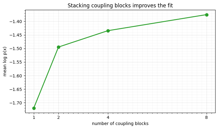
Likelihood climbs steadily with depth — one spline coupling can only do so much, but a stack composes them into the curved, non-separable map the spiral needs. The gains taper as the flow saturates the target. (This is the coupling analogue of RBIG’s depth, Part 3 — but here every block is trained jointly.)

2. Keeping a deep stack trainable¶

Depth has a cost: gradients flow through every block, and a long composition can amplify the occasional large update into a divergence. Well-conditioned stacks (the RQ-spline flows above, even at depth 20) train fine at a moderate learning rate, but push the rate up — or go deeper, or higher-dimensional — and stability tools earn their keep. The most reliable in our loop is gradient clipping (optax.clip_by_global_norm): it lets a deep affine stack (affine couplings are less self-stabilising than splines) survive an aggressive learning rate.

# Gradient norm of the NLL w.r.t. all parameters, for *untrained* stacks of growing
# depth — a training-free probe of how the composition amplifies gradients.
def grad_global_norm(flow):
    params, static = eqx.partition(flow, eqx.is_inexact_array)
    grads = eqx.filter_grad(
        lambda p: -jnp.mean(jax.vmap(eqx.combine(p, static).log_prob)(X[:1000])))(params)
    return float(optax.global_norm(grads))

stack_depths = [2, 4, 8, 16]
gn = {c: [grad_global_norm(build(jr.key(0), d, coupling=c)) for d in stack_depths]
      for c in ["affine", "spline"]}
for c in gn:
    print(f"  {c:7s} gradient norm at depths {stack_depths}: "
          + ", ".join(f"{x:.1f}" for x in gn[c]))

fig, ax = plt.subplots(figsize=(7.2, 4.3))
ax.plot(stack_depths, gn["spline"], "s-", color="tab:green", lw=2, ms=7, label="RQ-spline")
ax.plot(stack_depths, gn["affine"], "o-", color="tab:red", lw=2, ms=7, label="affine")
ax.set(title="Gradient norm grows with depth → deep stacks need a leash",
       xlabel="number of coupling blocks", ylabel="‖∇ NLL‖ (global norm)", xticks=stack_depths)
ax.legend(fontsize=9); style_ax(ax)
fig.tight_layout()

  affine  gradient norm at depths [2, 4, 8, 16]: 1.8, 3.6, 2.4, 8.9
  spline  gradient norm at depths [2, 4, 8, 16]: 3.1, 5.3, 7.7, 37.1

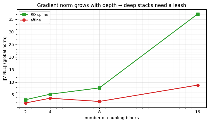
The gradient norm grows with depth — composing more blocks amplifies the back-propagated gradient (an order of magnitude over $2\to16$ blocks for the spline). With a fixed learning rate that means deeper stacks take ever-larger effective steps, so the occasional batch can blow training up. The standard guards:

Gradient clipping (optax.clip_by_global_norm, used throughout this part) caps that norm so depth cannot turn one bad batch into a NaN — cheap insurance that lets you train deep at an aggressive learning rate. (On the well-conditioned spline stacks of §1 a moderate rate already trains stably; the clip matters as you push rate, depth, or dimension.)
ActNorm pre-conditioning (Part 2 03) — a per-channel affine that normalises activations between blocks, the Glow stabiliser Kingma & Dhariwal (2018). It helps only when data-dependently initialised (loc/scale from the first batch); dropped in with default scale it compounds across depth and hurts, so it is a deliberate tool, not a free add-on.
RBIG warm-start (notebook 05) — starting at the diagonal RBIG solution sidesteps the worst of the from-scratch transient.

Together — alternating masks, clipping, ActNorm (data-initialised), and a warm start — these make very deep coupling flows trainable.

3. Residual coupling — a preview of implicit flows¶

Coupling gets its free log-det from a triangular Jacobian. A different family trades that for a residual map,

T(x) = x + g_\theta(x),

((1))

where $g_\theta$ is an unrestricted network (no split, no mask). This is more expressive per layer, but it is invertible only if $g_\theta$ is a contraction — $\mathrm{Lip}(g_\theta) < 1$ — and then it has no closed-form inverse: you recover $x$ from $y$ by Banach fixed-point iteration $x_{k+1} = y - g_\theta(x_k)$ . We illustrate the Lipschitz condition on a 1-D residual map $g(x)=a\sin(bx)$ .

xx = np.linspace(-3, 3, 400)

def banach_inverse(y, a, b, iters=60):
    x = np.array(y, dtype=float)
    for _ in range(iters):
        x = y - a * np.sin(b * x)
    return x

fig, axes = plt.subplots(1, 2, figsize=(11, 4.4), sharex=True, sharey=True)
for ax, (a, b) in zip(axes, [(0.3, 1.0), (0.9, 1.5)]):
    y = xx + a * np.sin(b * xx)
    lip = a * b
    mono = bool(np.all(np.diff(y) > 0))
    ax.plot(xx, y, color="tab:green" if mono else "tab:red", lw=2,
            label=f"$T(x)=x+{a}\\sin({b}x)$")
    ax.plot([-3, 3], [-3, 3], **GAUSS_KW, label="identity")
    if mono:
        rt = np.abs(xx - banach_inverse(y, a, b)).max()
        ax.text(-2.8, 3.0, f"Banach round-trip\nmax err {rt:.0e}", fontsize=8, color="tab:green")
    ax.set(title=f"Lip(g) = {lip:.2f} {'< 1 → invertible' if lip < 1 else '> 1 → not invertible'}",
           xlabel="x", ylim=(-4, 4))
    ax.legend(fontsize=8, loc="lower right"); style_ax(ax)
axes[0].set_ylabel("$T(x)$")
fig.suptitle("Residual map is invertible iff $g$ is a contraction", y=1.02)
fig.tight_layout()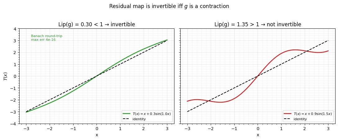

With $\mathrm{Lip}(g) = 0.3 < 1$ the map is monotone (invertible) and the fixed-point iteration recovers $x$ to machine precision; with $\mathrm{Lip} = 1.35

1$ the map folds over and is no longer a bijection. Residual flows (Behrmann

enforce the Lipschitz bound (spectral normalisation) and estimate the log-det with a Hutchinson power series — trading coupling’s free, exact machinery for more expressiveness per layer and an iterative inverse. That trade is the subject of Part 9 (relaxed-bijectivity and implicit flows).

Recap¶

knob	effect
depth (stacked blocks)	composes expressiveness; gains taper at saturation
gradient clipping	the reliable deep-stack stabiliser in our loop
ActNorm (data-init) / warm-start	further conditioning for deep flows
residual coupling $x+g(x)$	more expressive, but needs $\mathrm{Lip}(g)<1$ and an iterative inverse

Coupling flows scale by depth, and the coupling contract (triangular Jacobian, free log-det, exact inverse) survives every layer; residual flows give that contract up for raw expressiveness — a deliberate trade revisited in Part 9.

Part 5 → Part 6. That completes coupling-based Gaussianization: the pattern (00), bijector menu (01), conditioners (02), masks (03), the diagonal comparison and warm-start (04–05), the equivalence (06), and depth/stability here. Part 6 — Continuous-time Gaussianization takes the infinite-depth limit: instead of stacking discrete blocks, a flow ODE $\dot x = v_\theta(x,t)$ transports the data to $\mathcal{N}(0,I)$ continuously.

References¶

Kingma, D. P., & Dhariwal, P. (2018). Glow: Generative Flow with Invertible 1x1 Convolutions. Advances in Neural Information Processing Systems (NeurIPS).