Diagonal vs coupling marginal flows

04 — Diagonal vs coupling marginal flows¶

Notebooks 00–03 built the coupling machinery; now we put it head-to-head with the diagonal flow of Part 4. A diagonal flow rotates, then Gaussianizes each coordinate independently (gaussianization_flow) — all cross-coordinate modelling comes from stacking rotations, because the marginal step is separable. A coupling flow (coupling_gaussianization_flow) breaks that separability inside each layer (the pattern of notebook 00).

Is coupling genuinely more expressive, or does it just have more parameters? To answer fairly we compare the two at matched parameter count on a distribution built to need cross-coordinate structure: a spiral.

What you will see

The two factories: gaussianization_flow (diagonal) and coupling_gaussianization_flow (RQ-spline coupling) — and their very different per-layer parameter costs.
A likelihood-vs-parameters sweep: matched by parameters, the diagonal flow stays flat while a small-conditioner coupling already wins and improves with size.
The learned densities at comparable parameter counts: diagonal smears the spiral, coupling traces it.

import warnings

warnings.filterwarnings("ignore")

import equinox as eqx
import jax
import jax.numpy as jnp
import jax.random as jr
import matplotlib.pyplot as plt
import numpy as np
import optax

import gauss_flows as gf
from _style import SCATTER_KW, style_ax

jax.config.update("jax_enable_x64", True)
rng = np.random.default_rng(0)

# A two-arm spiral: strong nonlinear dependence between the coordinates.
n = 4000
t = rng.uniform(0.5, 3.5, n)
arm = (rng.integers(0, 2, n) * 2 - 1)[:, None]
xy = arm * np.stack([t * np.cos(2.5 * t), t * np.sin(2.5 * t)], axis=1)
xy = xy + 0.08 * rng.standard_normal((n, 2))
X = jnp.asarray((xy - xy.mean(0)) / xy.std(0))


def train_flow(flow, *, steps=1500, peak_lr=3e-3, clip_norm=1.0, batch=512, seed=1):
    """NLL training: optax with gradient clipping + one-cycle cosine LR."""
    params, static = eqx.partition(flow, eqx.is_inexact_array)
    schedule = optax.cosine_onecycle_schedule(transition_steps=steps, peak_value=peak_lr)
    opt = optax.chain(optax.clip_by_global_norm(clip_norm), optax.adam(schedule))
    state = opt.init(params)

    @eqx.filter_jit
    def step(params, state, xb):
        loss, grads = eqx.filter_value_and_grad(
            lambda p: -jnp.mean(jax.vmap(eqx.combine(p, static).log_prob)(xb)))(params)
        updates, state = opt.update(grads, state)
        return eqx.apply_updates(params, updates), state, loss

    key = jr.key(seed)
    for i in range(steps):
        key, sk = jr.split(key)
        idx = jr.randint(sk, (batch,), 0, X.shape[0])
        params, state, _ = step(params, state, X[idx])
    return eqx.combine(params, static)


logp = lambda flow: float(jax.vmap(flow.log_prob)(X).mean())
nparams = lambda flow: int(sum(x.size for x in jax.tree_util.tree_leaves(
    eqx.filter(flow, eqx.is_inexact_array))))

1. The two designs — and a fair comparison¶

Diagonal — gaussianization_flow(n_layers=L): $L$ blocks of (rotation → per-axis mixture-CDF Gaussianization). The marginal map factorises across coordinates; only the rotations mix them.
Coupling — coupling_gaussianization_flow(n_layers=L): $L$ blocks of rational-quadratic-spline coupling Durkan et al. (2019), where an MLP reads one half of the coordinates and outputs the spline parameters for the other half.

Comparing at equal layers would be unfair: a coupling layer carries an MLP conditioner, so with the default width it has ~100× more parameters than a diagonal layer. We instead compare at matched parameter count — shrinking the coupling conditioner (nn_width=16, nn_depth=1) and stacking more diagonal layers so the two live in the same budget range. (We cannot match exactly — the diagonal flow would need hundreds of layers to reach the coupling’s parameter counts — but we can overlap their ranges.)

diag = {L: gf.gaussianization_flow(jr.key(0), n_dims=2, n_layers=L, n_components=8)
        for L in [4, 8, 16]}
coup = {L: gf.coupling_gaussianization_flow(jr.key(0), n_dims=2, n_layers=L,
                                            n_bins=8, nn_width=16, nn_depth=1)
        for L in [2, 4, 8]}
print("parameter counts:")
print("  diagonal :", {L: nparams(f) for L, f in diag.items()})
print("  coupling :", {L: nparams(f) for L, f in coup.items()})

parameter counts:
  diagonal : {4: 212, 8: 420, 16: 836}
  coupling : {2: 1020, 4: 2036, 8: 4068}

2. Likelihood vs parameter count¶

We train every configuration with the same NLL optax loop and plot the held-out log-likelihood against the number of parameters — the fair axis. If parameters were all that mattered, the two curves would overlap.

trained_diag = {L: train_flow(f) for L, f in diag.items()}
trained_coup = {L: train_flow(f) for L, f in coup.items()}
for L, f in trained_diag.items():
    print(f"diagonal L={L:2d}: {nparams(f):5d} params -> log p {logp(f):.3f}")
for L, f in trained_coup.items():
    print(f"coupling L={L:2d}: {nparams(f):5d} params -> log p {logp(f):.3f}")

fig, ax = plt.subplots(figsize=(7.8, 4.6))
dp = np.array([(nparams(diag[L]), logp(trained_diag[L])) for L in diag])
cp = np.array([(nparams(coup[L]), logp(trained_coup[L])) for L in coup])
ax.plot(dp[:, 0], dp[:, 1], "o-", color="tab:blue", lw=2, ms=7, label="diagonal (per-axis marginal)")
ax.plot(cp[:, 0], cp[:, 1], "s-", color="tab:green", lw=2, ms=7, label="coupling (cross-coordinate)")
ax.set(title="Matched by parameters, coupling still wins on the spiral",
       xlabel="number of parameters (log scale)", ylabel="mean log p(x) (higher = better)",
       xscale="log")
ax.legend(fontsize=9); style_ax(ax)
fig.tight_layout()

diagonal L= 4:   212 params -> log p -2.710

diagonal L= 8:   420 params -> log p -2.732

diagonal L=16:   836 params -> log p -2.744

coupling L= 2:  1020 params -> log p -2.239
coupling L= 4:  2036 params -> log p -2.028

coupling L= 8:  4068 params -> log p -1.573

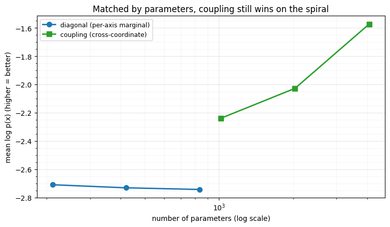
Even on the fair (per-parameter) axis the curves do not overlap. The diagonal flow is essentially flat around -2.7 across its whole range — more parameters (more layers) do not help it carve the spiral. The coupling flow, with a smaller conditioner than its default, already beats the diagonal flow at a comparable parameter count and keeps improving as it grows. So the win in expressiveness is not just “coupling has more knobs”: per parameter, the cross-coordinate conditioner is far more efficient at representing the spiral’s non-separable dependence.

3. The learned densities (comparable parameter counts)¶

We plot a diagonal and a coupling flow at similar parameter counts — diagonal $L=16$ vs coupling $L=2$ (both $\sim$ 900–1000 params) — the genuinely apples-to-apples picture.

diag_d, coup_d = trained_diag[16], trained_coup[2]
gx, gy = np.meshgrid(np.linspace(-2.5, 2.5, 120), np.linspace(-2.5, 2.5, 120))
grid = jnp.asarray(np.column_stack([gx.ravel(), gy.ravel()]))

fig, axes = plt.subplots(1, 3, figsize=(14.5, 4.6))
axes[0].scatter(X[:, 0], X[:, 1], color="tab:blue", **SCATTER_KW)
axes[0].set(title="data (spiral)", xlabel="$x_0$", ylabel="$x_1$")
for ax, model, t in [(axes[1], diag_d, f"diagonal (L=16, {nparams(diag_d)}p)"),
                     (axes[2], coup_d, f"coupling (L=2, {nparams(coup_d)}p)")]:
    lp = np.asarray(jax.vmap(model.log_prob)(grid)).reshape(gx.shape)
    ax.contourf(gx, gy, np.exp(lp), levels=18, cmap="viridis")
    ax.scatter(X[:, 0], X[:, 1], s=3, color="white", alpha=0.2)
    ax.set(title=f"{t}\nlog p = {logp(model):.2f}", xlabel="$x_0$")
for ax in axes:
    ax.set_aspect("equal"); style_ax(ax)
fig.suptitle("At comparable parameter counts: diagonal smears, coupling traces", y=1.02)
fig.tight_layout()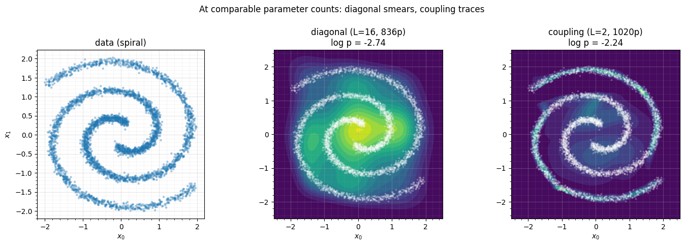

With essentially the same parameter budget, the diagonal flow still spreads probability into a loose blob while the coupling flow already bends along the arms. The conditioner is doing the work: it lets one coordinate’s transform depend on the other — the non-separability the spiral demands — and it does so far more economically than stacking separable layers.

Recap¶

design	per-layer map	cross-coordinate dependence	on the spiral (per parameter)
diagonal (`gaussianization_flow`)	per-axis mixture-CDF + rotation	only via stacked rotations	flat ~-2.7 regardless of size
coupling (`coupling_gaussianization_flow`)	RQ-spline, params from an MLP on the other half	within each layer	better at matched params, improves with size

Compared fairly by parameter count, coupling is the more expressive design for non-separable structure — not merely because it has more parameters. When the dependence is mild, the cheaper diagonal flow (and its RBIG warm-start) is plenty.

Next up. Coupling flows are expressive but harder to train from scratch. 05 — RBIG warm-start for coupling flows warm-starts one from a greedy RBIG fit via the zero-kernel contract — each coupling begins as a diagonal RBIG marginal, then training switches the conditioner on.

References¶

Durkan, C., Bekasov, A., Murray, I., & Papamakarios, G. (2019). Neural Spline Flows. Advances in Neural Information Processing Systems (NeurIPS).