Source

HSIC¶

We use the Hilbert-Schmidt Independence Criterion (HSIC) measure independence between two distributions. It involves constructing an appropriate kernel matrix for each dataset and then using the Frobenius Norm as a way to "summarize" the variability of the data. Often times the motivation for this method is lost in the notorious paper of Arthur Gretton (the creator of the method), but actually, this idea was developed long before him with ideas from a covariance matrix perspective. Below are my notes for how to get from a simple covariance matrix to the HSIC method and similar ones.

Motivation¶

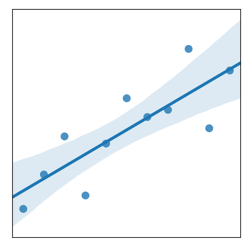
A very common mechanism to measure the differences between datasets is to measure the variability. The easiest way is the measure the covariance between the two datasets. However, this is limited to datasets with linear relationships and with not many outliers. Anscombe's classic dataset is an example where we have datasets with the same mean and standard deviation.



Case I	Case II	Case III	Case IV

This means measures like the covariance and correlation become useless because they will yield the same result. This requires us to have more robust methods that take into account the non-linear relationships that are clearly present within the data. That...or to do some really good preprocessing to make models easier.

Recap - Summarizing Multivariate Information¶

Let's have the two distributions $\mathcal{X} \in \mathbb{R}^{D_x}$ and $\mathcal{Y} \in \mathbb{R}^{D_y}$ . Let's also assume that we can sample $(x,y)$ from $\mathbb{P}_{xy}$ . We can capture the second order dependencies between $X$ and $Y$ by constructing a covariance matrix in the feature space defined as:

$C_{\mathbf{xy}} \in \mathbb{R}^{D \times D}$

We can use the Hilbert-Schmidt Norm (HS-Norm) as a statistic to effectively summarize content within this covariance matrix. It's defined as:

$||C_{xy}||_{\mathcal{F}}^2 = \sum_i \lambda_i^2 = \text{tr}\left[ C_{xy}^\top C_{xy} \right]$

Note that this term is zero iff $X$ and $Y$ are independent and greater than zero otherwise. Since the covariance matrix is a second-order measure of the relations, we can only summarize the the second order relation information. But at the very least, we now have a scalar value that summarizes the structure of our data.

And also just like the correlation, we can also do a normalization scheme that allows us to have an interpretable scalar value. This is similar to the correlation coefficient except it can now be applied to multi-dimensional data.

$\rho_\mathbf{xy} = \frac{ ||C_{\mathbf{xy}}||_\mathcal{F}^2}{||C_\mathbf{xx}||_{\mathcal{F}} ||C_\mathbf{yy}||_{\mathcal{F}}}$

Samples versus Features¶

One interesting connection is that using the HS norm in the feature space is the sample thing as using it in the sample space.

$\langle C_{\mathbf{x^\top y}}, C_{\mathbf{x^\top y}}\rangle_{\mathcal{F}} = \langle C_{\mathbf{xx^\top }}, C_{\mathbf{yy^\top}}\rangle_{\mathcal{F}}$

Comparing Features is the same as comparing samples!

Note: This is very similar to the dual versus sample space that is often mentioned in the kernel literature.

So our equations before will change slightly in notation as we are constructing different matrices. But in the end, they will have the same output. This includes the correlation coefficient $\rho$ .

$\frac{\langle C_{\mathbf{x^\top y}}, C_{\mathbf{x^\top y}}\rangle_{\mathcal{F}}}{||C_\mathbf{x^\top x}||_{\mathcal{F}} ||C_\mathbf{y^\top y}||_{\mathcal{F}}} = \frac{ \langle C_{\mathbf{xx^\top }}, C_{\mathbf{yy^\top}}\rangle_{\mathcal{F}}}{||C_\mathbf{xx^\top}||_{\mathcal{F}} ||C_\mathbf{yy^\top}||_{\mathcal{F}}}$

Kernel Trick¶

So now, we have only had a linear dot-similarity in the sample space of $\mathcal{X}$ and $\mathcal{Y}$ . This is good but we can easily extend this to a non-linear transformation where we add an additional function $\psi$ for each of the kernel functions.

$\langle C_{\mathbf{xx^\top }}, C_{\mathbf{yy^\top}}\rangle_{\mathcal{F}} = \langle K_{\mathbf{x}}, K_{\mathbf{y}}\rangle_\mathcal{F}$

Let's assume there exists a nonlinear mapping from our data space to the Hilbert space. So $\phi : \mathcal{X} \rightarrow \mathcal{F}$ and $\psi : \mathcal{Y} \rightarrow \mathcal{G}$ . We also assume that there is a representation of this mapping via the dot product between the features of the data space; i.e. $K_x(x,x') = \langle \phi(x), \phi(x') \rangle$ and $K_y(y,y') = \langle \psi(y), \psi(y') \rangle$ . So now the data matrices are $\Phi \in \mathbb{R}^{N\times N_\mathcal{F}}$ and $\Psi \in \mathbb{R}^{N \times N_\mathcal{G}}$ . So we can take the kernelized version of the cross covariance mapping as defined for the covariance matrix:

$\begin{aligned} ||C_{\phi(x)\psi(x)}||_\mathcal{H}^2 &= ||\Phi^\top \Psi||^2_{\mathcal{F}} \end{aligned}$

Now after a bit of simplication, we end up with the HSIC-Norm:

$\begin{aligned} \text{HSIC}(\hat{P}_{XY}, \mathcal{F}, \mathcal{G}) &= \text{Tr}(K_{\mathbf{x}}K_{\mathbf{y}}) \\ \end{aligned}$

Details

Proof

$\begin{aligned} ||C_{\phi(x)\psi(x)}||_\mathcal{H}^2 &= ||\Phi^\top \Psi||^2 \\ &= tr\left[ (\Phi^\top \Psi)^\top (\Phi^\top \Psi)\right] \\ &= tr \left[ \Psi^\top \Phi \Phi^\top \Psi\right] \\ &= tr \left[ \Psi \Psi^\top \Phi \Phi^\top \right] \\ &= tr (K_{\mathbf{x}}K_{\mathbf{x}}) \end{aligned}$

Full Expression

Using the same argument as above, we can also define a cross covariance matrix of the form:

$C_{xy} = \mathbb{E}_{xy} \left[ (\phi(x) - \mu_x) \otimes (\psi(y) - \mu_y)\right]$

where $\otimes$ is the tensor product, $\mu_x, \mu_y$ are the expecations of the mappings $\mathbb{E}_x [\phi (x)]$ , $\mathbb{E}_y[\psi(y)]$ respectively. The HSIC is the cross-covariance operator described above and can be expressed in terms of kernels.

$\begin{aligned} \text{HSIC}(\mathcal{F}, \mathcal{G}, \mathbb{P}_{xy}) &= ||C_{xy}||_{\mathcal{H}}^2 \\ &= \mathbb{E}_{xx',yy'} \left[ K_x(x,x')K_y(y,y') \right] \\ &+ \mathbb{E}_{xx'} \left[ K_x(x,x')\right] \mathbb{E}_{yy'} \left[ K_y(y,y')\right] \\ &- 2\mathbb{E}_{xy} \left[ \mathbb{E}_{x'} \left[ K_x(x,x')\right] \mathbb{E}_{y'} \left[ K_y(y,y')\right] \right] \end{aligned}$

where $\mathbb{E}_{xx'yy'}$ is the expectation over both $(x,y) \sim \mathbb{P}_{xy}$ and we assume that $(x',y')$ can be sampled independently from $\mathbb{P}_{xy}$ .

Code

This is very easy to compute in practice. One just needs to calculate the Frobenius Norm (Hilbert-Schmidt Norm) between two kernel matrics that correctly model your data. This boils down to computing the trace of the matrix multiplication of two matrices: $tr(K_x^\top K_y)$ . So in algorithmically that is

hsic_score = np.trace(K_x.T @ K_y)

Notice that this is a 3-part operation. So, of course, we can refactor this to be much easier. A faster way to do this is:

hsic_score = np.sum(K_x * K_y)

This can be orders of magnitude faster because it is a much cheaper operation to compute elementwise products than a sum. And for fun, we can even use the einsum notation.

hsic_score = np.einsum("ji,ij->", K_x, K_y)

Centering¶

A very important but subtle point is that the method with kernels assumes that your data is centered in the kernel space. This isn't necessarily true. Fortunately it is easy to do so.

$HK_xH = \tilde{K}_x$

where $H$ is your centering matrix.

Normalizing your inputs does not equal centering your kernel matrix.

Details

Full Expression

We assume that the kernel function $\psi(x_i)$ has a zero mean like so:

$\psi(x_i) = \psi(x_i) - \frac{1}{N}\sum_{r=1}^N \psi(x_r)$

This holds if the covariance matrix is computed from $\psi(x_i)$ . So the kernel matrix $K_{ij}=\psi(x_i)^\top \psi(x_j)$ needs to be replaced with $\tilde{K}_{ij}=\psi(x_i)^\top \psi(x_s)$ where $\tilde{K}_{ij}$ is:

$\begin{aligned} \tilde{K}_{ij} &= \psi(x_i)^\top \psi(x_j) - \frac{1}{N} \sum_{r=1}^N - \frac{1}{N} \sum_{r=1}^N \psi(x_r)^\top \psi(x_j) + \frac{1}{N^2} \sum_{r,s=1}^N \psi(x_r))^\top \psi(x_s) \\ &= K_{ij} - \frac{1}{N}\sum_{r=1}^{N}K_{ir} - \frac{1}{N} K_{rj} + \frac{1}{N^2} \sum_{r,s=1}^N K_s \end{aligned}$

Code

On a more practical note, this can be done easily by:

$H = \mathbf{I}_N - \frac{1}{N} \mathbf{1}_N\mathbf{1}_N^\top$

H = np.eye(n_samples) - (1 / n_samples) * np.ones(n_samples, n_samples)

Refactor

There is also a function in the scikit-learn library which does it for you.

from sklearn.preprocessing import KernelCenterer

K_centered = KernelCenterer().fit_transform(K)

Correlation¶

So above is the entire motivation behind HSIC as a non-linear covariance measure. But there is the obvious extension that we need to do: as a similarity measure (i.e. a correlation). HSIC suffers from the same issue as a covariance measure: it is difficult to interpret. HSIC's strongest factor is that it can be used for independence testing. However, as a similarity measure, it violates some key criteria that we need: invariant to scaling and interpretability (bounded between 0-1). Recall the HSIC formula:

$A(K_x, K_y) = \left\langle H K_x, H K_y \right\rangle_{F}$

Below is the HSIC term that is normalized by the norm of the

$\text{cKA}(\mathbf{xy})=\frac{ \langle K_{\mathbf{x}}, K_{\mathbf{y}}\rangle_\mathcal{F}}{||K_\mathbf{x}||_{\mathcal{F}} ||K_\mathbf{y}||_{\mathcal{F}}}$

This is known as Centered Kernel Alignment in the literature. They add a normalization term to deal with some of the shortcomings of the original Kernel Alignment algorithm which had some benefits e.g. a way to cancel out unbalanced class effects. In relation to HSICThe improvement over the original algorithm seems minor but there is a critical difference. Without the centering, the alignment does not correlate well to the performance of the learning machine. There is

Original Kernel Alignment

The original kernel alignment method had the normalization factor but the matrices were not centered.

$A(K_x, K_y) = \frac{\left\langle K_x, K_y \right\rangle_{F}}{\sqrt{|| K_x||_{F}|| K_y ||_{F}}}$

The alignment can be seen as a similarity score based on the cosine of the angle. For arbitrary matrices, this score ranges between -1 and 1. But using positive semidefinite Gram matrices, the score is lower-bounded by 0. This method was introduced before the HSIC method was introduced by Gretton. However, because the kernel matrices were not centered, there were some serious problems when trying to use it for measuring similarity: You could literally get any number between 0-1 if with parameters. So for a simple 1D linear dataset which should have a correlation of 1, I could get any number between 0 and 1 if I just change the length scale slightly. The HSIC and the CKA were much more robust than this method so I would avoid it.

Connections¶

Maximum Mean Discrepency¶

HSIC

$\text{MMD}^2(\hat{P}_{XY}, \hat{P}_X\hat{P}_Y, \mathcal{H}_k) = \frac{1}{n^2}\text{tr} \left( K_x H K_y H \right)$

where $H$ is the centering matrix $H=I_n-\frac{1}{n}1_n1_n^\top$ .

$\text{HSIC}^2(\hat{P}_{XY}, \mathcal{F}, \mathcal{G}) = \text{MMD}^2(\hat{P}_{XY}, \hat{P}_X\hat{P}_Y, \mathcal{H}_k)$

$\text{HSIC}_k(\mathbb{P}) = \text{MMD}_k(\mathbb{P}, \otimes_{m=1}^M \mathbb{P}_m)$

Information Theory Measures¶

Kullback-Leibler Divergence

$D_{KL}(\mathbb{P}, \mathbb{Q}) = \int_{\mathbb{R}^d} p(x) \log \left[ \frac{p(x)}{q(x)} \right]dx$

Mutual Information

$I(\mathbb{P})=D_{KL}\left( \mathbb{P}, \otimes_{m=1}^{M}\mathbb{P}_m \right)$

Future Outlook¶

Advantages

Sample Space - Nice for High Dimensional Problems w/ a low number of samples
HSIC can estimate dependence between variables of different dimensions
Very flexible: lots of ways to create kernel matices

Disadvantages

Computationally demanding for large scale problems
Non-iid samples, e.g. speech or images
Tuning Kernel parameters
Why the HS norm?

Resources¶

Presentations

HSIC, A Measure of Independence - Szabo (2018)
Measuring Independence with Kernels - Gustau

Literature Review¶

An Overview of Kernel Alignment and its Applications - Wang et al (2012) - PDF

This goes over the literature of the kernel alignment method as well as some applications it has been used it.

Applications¶

Kerneel Target Alignment Parameter: A New Modelability for Regression Tasks - Marcou et al (2016) - Paper
Brain Activity Patterns - Paper
Scaling - Paper

Textbooks¶

Kernel Methods for Digital Processing - Book