GPs and Uncertain Inputs through the Ages
Summary
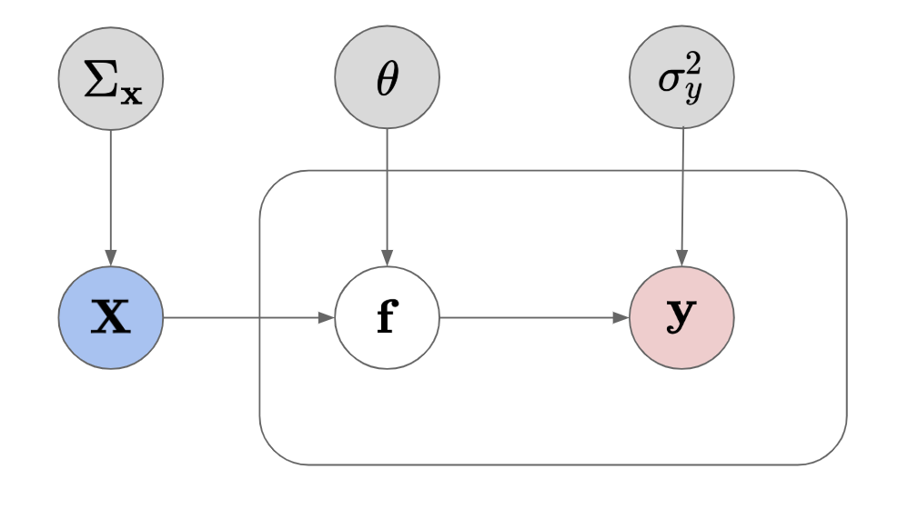 |
Figure: Intuition of a GP which takes into account the input error.
When applying GPs for regression, we always assume that there is noise \sigma_y^2 in the output measurements \mathbf y. We rarely every assume that their are errors in the input points \mathbf x. This assumption does not hold as we can definitely have errors in the inputs as well. For example, most sensors that take measurements have well calibrated errors which is needed for inputs to the next model.
This chain of error moving through models is known as error propagation; something that is well known to any physics 101 student that has ever taken a laboratory class. In this review, I would like to go through some of the more important algorithms and dissect some of the mathematics behind it so that we can arrive at some understanding of uncertain inputs through the ages with GPs.
As a quick overview, we will look at the following scenarios:
- Stochastic Test Data
- Stochastic Input Data
- My Contribution
Standard GP Formulation
Given some data \mathcal{D}(X,y) we want to learn the following model.
So remember, we have the following 3 important quantities:
- Gaussian Likelihood: \mathcal{P}(y|\mathbf{x}, f) \sim \mathcal{N}(f, \sigma_y^2\mathbf I)
- Gaussian Process Prior: \mathcal{P}(f) \sim \mathcal{GP}(\mathbf m, \mathbf K_\theta)
- Gaussian Posterior: \mathcal{P}(f|\mathbf{x}, y) \sim \mathcal{N}(\mu, \mathbf \nu^2)
If you go through the steps of the GP formulation (see other document), then you will arrive at the following predictive distribution:
where:
This is the typical formulation which assumes that the output of x is deterministic. However, what happens when x is stochastic with some noise variance? We want to account for this in our scheme.
Source: * Rasmussen - GPs | GP Posterior | Marginal Likelihood
Stochastic Test Points
This is the typical scenario for most of the methods that exist in todays literature (that don't involve variational inference). In this instance, we are looking mainly at noisy test data \mathbf X_*. This is where most of the research lies as it is closely related to dynamical systems. Imagine you have some function with respect to time
At time step t=0 we will have some output x_{1} which is subject to f_0(x_0) and \epsilon_0. The problem with this is that now the next input at time t=1 is a noisy input; by definition f_1(\mathbf x_1 + \epsilon_1). So we can easy imagine how this subsequent models t+1 can quickly decrease in accuracy because the input error is now un-modeled.
In the context of GPs, if a test input point \mathbf x_* has noise, we can simply integrate over all possible trial points. This will not result in a Gaussian distribution. However, we can approximate this distribution as Gaussian using moment matching methods by analytically (or numerically) calculating the mean and covariance.
Setup
Let's define the model under the assumption that \mathbf{\bar{x}} are noise-free inputs to the f(\cdot). With equations that looks something like:
I've summarized the terms of these equations in words below:
Equation I - Training Time
- y - noise-corrupted training outputs
- \mathbf{x} - noise-free training inputs
- f(\cdot, \theta) - function parameterized by \theta
- \epsilon_y \sim \mathcal{N}(0, \sigma^2_y)
Equation II - Testing Time
- y_* - noise-corrupted test outputs
- \mathbf x_* - noise-corrupted test inputs
- f(\cdot, \theta) - function parameterized by \theta
- \epsilon_y \sim \mathcal{N}(0, \sigma^2_y)
Equation III - Test Inputs Relationship
- \mathbf x_* - noise-corrupted test inputs
- \mathbf{\bar x}_* - noise-free test inputs
- \epsilon_x \sim \mathcal{N}(0, \Sigma_x)
It seems like a lot of equations but I just wanted to highlight the distinction between the training procedure where we assume the inputs are noise-free and the testing procedure where we assume the inputs are noisy. Immediately this does not seem correct and we can immediately become skeptical at this decision but as a first approximation (especially applicable to time series), this is a good first step.
GP Predictive Distribution
So assuming that we are OK with this assumption, we can move on and think of this in terms of GPs. The nice thing about this setup is that we only need to care about the posterior of the GP because it only has an influence at test time. So we can train a GP assuming that the points that are being used for training are noise-free.
More concretely, let's look at the only function that really matters in this scenario: the posterior function for a GP:
Throughout this whole equation we have \mathbf x_* \sim \mathcal{N}(\bar{\mathbf x}_*, \Sigma_{x*}). This implies that \mathbf x_* is no longer deterministic; we now have a conditional distribution \mathcal{P}(f_*|\mathbf x_*). We are not interested in this conditional probability distribution, only in the probability distribution of f_*, \mathcal{P}(f_*). So, to get rid of the \mathbf x_*'s, we need to integrate them out. Through marginalization, we get the predictive distribution for f_* by this equation:
(I omitted the conditional dependency on \mathcal{D}, \mathbf x_* and \theta for brevity). We assume that \mathbf x_* is normally distributed and f_* is normally distributed. So that means the conditional distribution \mathcal{P}(f_* | \mathbf x_*) is also normally distributed. The problem is that integrating out the \mathbf x_* it's not tractable. For example, for the first term (the most problematic) in the integral equation above we have:
It's not trivially how to find the determinant nor the inverse of the variance term inside of the equation.
Numerical Integration
The immediate way of solving some complex integral is to just brute force it with something like Monte-Carlo.
where every x_*^t is drawn from \mathcal{N}(\bar{\mathbf x}_*|\Sigma_x). This will move towards the true distribution as T gets larger but it can be prohibitive when dealing with high dimensional spaces as thee time need to converge to the true distribution gets longer as well. To get an idea about how this works, we can take a look using a simple numerical calculation (example).
Approximate Gaussian Distribution
Another problem is that the resulting distribution may not result in a Gaussian distribution (due to some nonlinear interactions within the terms). We want it to be Gaussian because they're easy to use so it's in our best interest that they're Guassian. We could use Gaussian mixture models or Monte Carlo methods to deal with the non-Gaussian distributions. But in most of the literature, you'll find that we want assume (or force) the distribution to Gaussian by way of moment matching. For any distribution to be approximated as a Gaussian, we just need the expectation \mathbb{E}[f_*] and the variance \mathbb{V}[f_*] of that distribution. The derivation is quite long and cumbersome so I will skip to the final formula:
where \mathbf \Omega is something we call a kernel expectation (or sufficient statistic) in some cases. This involves the expectation given some distribution (usually the Normal distribution) where you need to integrate out the inputs. There are closed forms for some of these with specific kernels (see suppl. section below) but I will omit this information in this discussion.
Overall the expression obtained above is a familiar expression with some different parameters. We can calculate the variance using some of the same logic but it's not as easy. So, to save time, I'll skip to the final part of the equation because the derivation is even worse than the mean.
where \xi and \Phi are also kernel expectations. This final expression is not intuitive but it works fine for many applications; most notably the PILCO problem. The derivation in its entirety can be found here, here, and here if you're interested. It's worth noting that I don't this method is suitable for big data without further approximations to the terms in this equation as at first site it looks very inefficient and with complex and expensive calculations.
Stochastic Measurements
A different; and perhaps more realistic and useful scenario; is if we assume that all of the inputs are stochastic. If all input points X are stochastic, the above techniques of moment matching don't work well because typically they only look at test time and not training time. So, again, let's redefine the model under the assumption that \mathbf x \sim \mathcal{N}(\bar{\mathbf{x}}, \Sigma_x). With equations that look something like:
where:
- y - noise-corrupted outputs
- f(\cdot, \theta) - function parameterized by \theta
- \epsilon_y \sim \mathcal{N}(0, \sigma^2_y)
- \mathbf x - noise-corrupted training inputs
- \mathbf{\bar x} - noise-free training inputs
- \epsilon_x \sim \mathcal{N}(0, \Sigma_x)
So in this scenario, we find that the training points are stochastic and the test points are deterministic. This gives us problems when we try to use the same techniques as mentioned above. As an example, let's look at the posterior function for a GP except it doesn't have to be at test time:
We can skip all of that from the first section because we are assuming that \mathbf x_* is deterministic (????). We have to remember that we are assuming that we've already found the parameters \bar{\mathbf{x}} and \Sigma_\mathbf{x}. So we just need to try and see if we can calculate the \mu_* and \nu^2_*. To see why it's not really possible to marginalize by the inputs, let's try to calculate the posterior mean \mu_*. This equation depends on \mathbf x_* and \mathbf x where \mathbf x\sim \mathcal{N}(\bar{\mathbf x}, \Sigma_x). So if we want to marginalize over all of the stochastic data we get:
Now the integral of the first term alone \mu(\mathbf x_*|\mathbf x) is a non-trivial integral especially for the inverse of the kernel matrix \mathbf K which does not have a trivial solution. So just looking at the posterior function alone, there are problems with this approach. We will have to somehow augment our function to account for this problem. Below, we will discuss an algorithm that attempts to remedy this.
Noisy-Input GP (NIGP)
We're going to make a slight modification to the above equation for stochastic measurements. We will keep the same assumption of stochastic measurements, \mathbf x \sim \mathcal{N}(\bar{\mathbf{x}}, \Sigma_x). It doesn't change the properties of the formulation but it does change the perspective.
where:
- y - noise-corrupted outputs
- f(\cdot, \theta) - function parameterized by \theta
- \epsilon_y \sim \mathcal{N}(0, \sigma^2_y)
- \mathbf x - noise-corrupted training inputs
- \mathbf{\bar x} - noise-free training inputs
- \epsilon_x \sim \mathcal{N}(0, \Sigma_x)
The definitions are exactly the same but we need to think of the model itself as having the \mathbf x - \epsilon_x as the input to the latent function f. Rewriting this expression does not solve the problem as we would still have difficulties marginalizing by the stochastic inputs. Instead, the author uses a first order Taylor series approximation of the GP latent function f w.r.t. \mathbf x to separate the terms which allows us to have an easier function to approximate. We end up with the following equation:
where:
- y - noise-corrupted outputs
- f(\cdot, \theta) - function parameterized by \theta
- \epsilon_y \sim \mathcal{N}(0, \sigma^2_y)
- \frac{\partial f (\cdot)}{\partial x} - the derivative of the latent function f w.r.t. \mathbf x
- \mathbf x - noise-corrupted training inputs
- \epsilon_x \sim \mathcal{N}(0, \Sigma_x)
We have replaced our \mathbf{\bar x} with a new derivative term and these brings in some new ideas and questions: what does this mean to have the derivative of our latent function and how does relate to the error in our latent function f?

Figure: Intuition of the NIGP:
- a) y=f(\mathbf x) + \epsilon_y
- b) y=f(\mathbf x + \epsilon_x)
- c) y=f(\mathbf x + \epsilon_x) + \epsilon_y
The key idea to think about is what contributes to how far away the error bars are from the approximated mean function. The above graphs will help facilitate the argument given below. There are two main components:
- Output noise \sigma_y^2 - the further away the output points are from the approximated function will contribute to the confidence intervals. However, this will affect the vertical components where it is flat and not so much when there is a large slope.
- Input noise \epsilon_x - the influence of the input noise depends on the slope of the function. i.e. if the function is fully flat, then the input noise doesn't affect the vertical distance between our measurement point and the approximated function; contrast this with a function fully sloped then we have a high contribution to the confidence interval.
So there are two components of competing forces: \sigma_y^2 and \epsilon_x and the \epsilon_x is dependent upon the slope of our function \partial f(\cdot) w.r.t. \mathbf x. So, getting back to our Taylor expanded function which encompasses this relationship, we will notice that it is not a Gaussian distribution because of the product of the Gaussian vector \epsilon_x and the derivative of the GP function (it is Gaussian, just not a Gaussian PDF). So we will have problems with the inference so we need to make approximations in order to use standard analytical methods. The authors outline two different approaches which we will look at below; they have very similar outcomes but different reasonings.
Expected Derivative
Remember a GP function is defined as : f \sim \mathcal{GP}(\mu, \nu^2)
It's a random function defined by it's mean and variance. We can also write the derivative of a GP as follows:
Remember the derivative of a GP is still a GP so the treatment is the same. They suggest we take the expectation over the GP uncertainty, \mathbb{E}_f\left[ \frac{\partial f(\mathbf x)}{\partial x} \right] kind of acting as a first order approximation to the approximation. This equation now becomes Gaussian distributed which means we are simply adding a GP and a Gaussian distribution which is a Gaussian distribution (\mathcal{G} + \mathcal{GP}=\mathcal{G})(????). Taking the expectation over that GP derivative gives us the mean which is defined as the posterior mean of a GP.
So to take the expectation for the derivative of a GP would be taking the derivative w.r.t. to the posterior mean function, \partial\mu(\mathbf x) only. So in this instance, we just slightly modified our original equation so that we just need to take the derivative of the GP posterior mean instead of the whole distribution. So now we have a new likelihood function based on this approach of expectations:
where \tilde \Sigma_{\mathbf x}=\partial{\bar{f}}^{\top}\Sigma_x\partial{\bar{f}}.
Note: please see the supplementary section for a quick alternative explanation using ideas from the propagation of variances.
Moment Matching
The alternative and more involved approach is to use the moment matching approach again. We use this to compute the moments of this formulation to recover the mean and variance of this distribution. The first moment (the mean) is given by:
We still recover the GP prior mean which is the same for the standard GP. The variance is more difficult to calculate and I will omit most of the details as it can get a bit cumbersome.
and using some of the notation above, we can simplify this a bit:
You're more than welcome to read the thesis which goes through each term and explains how to compute the mean and variance for the derivative of a GP. The expression gets long but then a lot of terms go to zero. I went straight to the punchline because I think that's the most important part to take away. So to wrap it up and be consistent, the new likelihood function for the momemnt matching approach is:
where \tilde \Sigma_{\mathbf x}=\partial{\bar{f}}^{\top}\Sigma_x\partial{\bar{f}}. Right away you'll notice some similarities between the expectation versus the moment matching approach and that's the variance term \text{tr} \left( \Sigma_x\mathbb{V}_f\left[ \frac{\partial f(\mathbf x)}{\partial x} \right]\right) which represents the uncertainty in the derivative as a corrective matrix. Both the authors of the NIGP paper and the SONIG paper both confirm that this additional correction term has a negligible effect on the final result. It's also not trivial to calculate so the code-result ratio doesn't seem worthwhile in my opinion for small problems. This might make a difference in large problems and possibly higher dimensional data.
So the final formulation that we get for the posterior is:
The big problem with this approach is that we do not know the function f(\cdot) that we are approximating which means we cannot know the derivative of that function. So we are left with a recursive system where we need to know the function to calculate the derivative and we need to know the derivative to calculate the outputs. The solution is to use multiple iterations which is what was done in the NIGP paper (and similarly in the online version SONIG). Regardless, we are trying to marginalize the log likelihood. The likelihood is given by the normal distribution:
where \mathcal{K}_\theta=\mathbf K + \mathbf{\tilde \Sigma_\mathbf{x}} + \sigma^2_y \mathbf I. But we need to do a two-step procedure:
- Train a standard GP (with params \mathbf K + \sigma^2_y \mathbf I)
- Evaluate the Derivative terms with the GP (\partial{\bar f})
- Add the corrective term (\mathbf{\tilde \Sigma_\mathbf{x}}).
- Train the GP with the corrective terms (\mathbf K + \mathbf{\tilde \Sigma_\mathbf{x}} + \sigma^2_y \mathbf I).
- Repeat 2-4 until desired convergence.
TODO: My opinion.
Variational Strategies
What links all of the strategies above is how they approach the problem of uncertain inputs: approximating the posterior distribution. The methods that use moment matching on stochastic trial points are all using various strategies to construct some posterior approximation. They define their GP model first and then approximate the posterior by using some approximate scheme to account for uncertainty. The NIGP however does change the model which is a product of the Taylor series expansion employed. From there, the resulting posterior is either evaluated or further approximated. My method actually is related because I also avoid changing the model and just attempt approximate the posterior predictive distribution by augmenting the variance method only (???).
My Method - Marriage of Two Strategies
I looked at both strategies of stochastic trial points versus stochastic inputs to see how would it work in real applications. One thing that was very limiting in almost all of these methods was how expensive they were. When it comes to real data, calculating higher order derivatives can be very costly. It seemed like the more sophisticated the model, the more expensive the method is. An obvious example the NIGP where it requires multiple iterations in conjunction with multiple restarts to avoid local minimum. I just don't see it happening when dealing with 2,000+ points. However, I support the notion of using posterior information by the use of gradients of the predictive mean function as I think this is valuable information which GPs give you access to. With big data as my limiting factor, I chose to keep the training procedure the same but modify the predictive variance using the methodology from the NIGP paper. I don't really do anything new that cannot be found from the above notions but I tried to take the best of both worlds given my problem. I briefly outline it below.
Model
Using a combination of two strategies that we mentioned above:
- Stochastic trial points
- Derivative of the posterior mean function.
It's using the NIGP reasoning but with assuming only the trial points are stochastic. Let's define the model under the assumption that \mathbf{\bar{x}} are noise-free inputs to the f(\cdot). With equations that looks something like:
where only \mathbf x_* \sim \mathcal{N}\left(\mathbf{\bar x_*}, \Sigma_x \right) and \mathbf x is deterministic.
Inference
So the exact same strategy as listed above. Now we will add the final posterior distribution that we found from the NIGP but only for the test points:
In my work, I really only looked at the variance function to see if it was different. It didn't make sense to use the mean function with a different learning strategy. In addition, I found that the weights calculated with the correction were almost the same and I didn't see a real difference in accuracy for the experiments I conducted. So, to be complete, we come across my final algorithm:
I did an experiment where I was trying to predict temperature from radiances for some areas around the globe where the radiances that I received had known input errors. So I used those but only for the predictions. I found that the results I got for this method did highlight some differences in the variance estimates. If you try to correlate the standard deviation of the NIGP method versus the standard deviation from the standard GP, you get a very noticeable difference (see suppl. section below). The results were so convincing that I decided to take my research further in order to investigate some other strategies in order to account for input errors. One immediate obvious change is I could use the sparse GP approximation. But I think the most promising one that I would like to investigate is using variational inference which I outline in another document.
Source: * Accounting for Input Noise in GP Parameter Retrieval - letter
Supplementary Material
Moment Matching
In a nutshell, we can calculate the approximations of any distribution f by simply taking the moments of that distribution. Each moment is defined by an important statistic that most of us are familiar with:
- Mean, \mathbb{E}[f]
- Variance, \mathbb{V}[f]
- Skew, \mathbb{S}[f]
- Kurtosis, \mathbb{K}[f]
- Higher moments...
With each of these moments, we are able to approximate almost any distribution. For a Gaussian distribution, it can only be defined by the first and second moment because all of the other moments are zero. So we can approximate any distribution as a Gaussian by simply taking the expected value and the variance of that probability distribution function.
Kernel Expectations
So [Girard 2003] came up with a name of something we call kernel expectations \{\mathbf{\xi, \Omega, \Phi}\}-statistics. These are basically calculated by taking the expectation of a kernel or product of two kernels w.r.t. some distribution. Typically this distribution is normal but in the variational literature it is a variational distribution. The three kernel expectations that surface are:
To my knowledge, I only know of the following kernels that have analytically calculated sufficient statistics: Linear, RBF, ARD and Spectral Mixture. And furthermore, the connection is how these kernel statistics show up in many other GP literature than just uncertain inputs of GPs; for example in Bayesian GP-LVMs and Deep GPs.
Propagation of Variances
Let's reiterate our problem statement:
where:
- y - noise-corrupted outputs
- f(\cdot, \theta) - function parameterized by \theta
- \epsilon_y \sim \mathcal{N}(0, \sigma^2_y)
- \mathbf x - noise-corrupted training inputs
- \mathbf{\bar x} - noise-free training inputs
- \epsilon_x \sim \mathcal{N}(0, \Sigma_x)
First order Taylor Series expansion of f(x).
NIGP - Propagating Variances
Another explanation of the rational of the Taylor series for the NIGP stems from the error propagation law. Let's take some function f(\mathbf x) where x \sim \mathcal{P} described by a mean \mu_\mathbf{x} and covariance \Sigma_\mathbf{x}. The Taylor series expansion around the function f(\mathbf x) is:
This results in a mean and error covariance of the new distribution \mathbf z defined by:
I've linked a nice tutorial for propagating variances below if you would like to go through the derivations yourself. We can relate the above formula to the logic of the NIGP by thinking in terms of the derivatives (slopes) and the input error. We can actually calculate how much the slope contributes to the noise in the error in our inputs because the derivative of a GP is still a GP. Like above, assume that our noise \epsilon_x comes from a normal distribution with variance \Sigma_x, \epsilon_x \sim \mathcal{N}(0, \Sigma_x). We also assume that the slope of our function is given by \frac{\partial f}{\partial x}. At every infinitesimal point we have a tangent line to the slope, so multiplying the derivative by the error will give us an estimate of how much our variance estimate should change, \epsilon_x\frac{\partial f}{\partial x}. We've assumed a constant slope so we will have a mean of 0,
Now we just need to calculate the variance which is given by:
So we can replace the \epsilon_y^2 with a new estimate for the output noise:
And we can add this to our formulation:
Source:
- An Introduction to Error Propagation: Derivation, Meaning and Examples - Doc
- Shorter Summary - 1D, 2D Example
- Statistical uncertainty and error propagation
Real Results with Variance Estimates
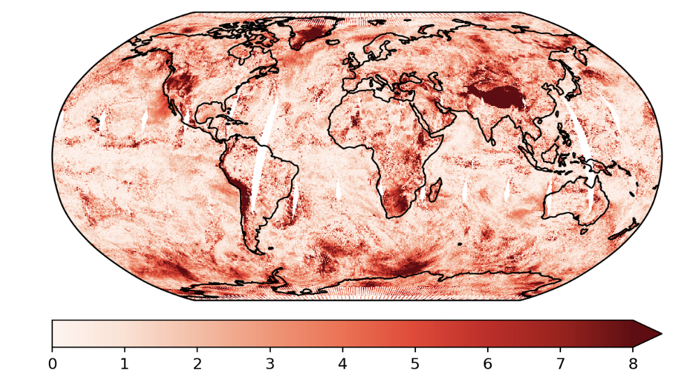
Figure: Absolute Error From a GP Model
These are the predictions using the exact GP and the predictive variances.
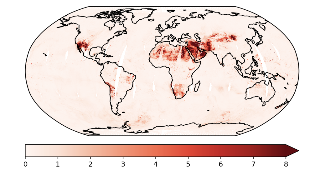
Figure: Standard GP Variance Estimates
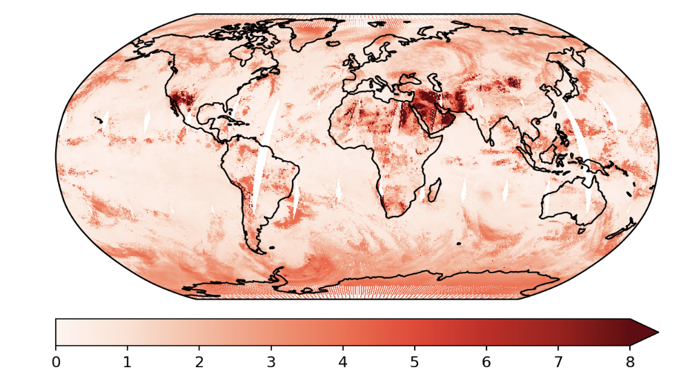
Figure: GP Variance Estimates account for input errors.
This is an example where we used the Taylor expanded GP. In this example, we only did the first order approximation.
Resources
Papers
Thesis Explain
Often times the papers that people publish in conferences in Journals don't have enough information in them. Sometimes it's really difficult to go through some of the mathematics that people put in their articles especially with cryptic explanations like "it's easy to show that..." or "trivially it can be shown that...". For most of us it's not easy nor is it trivial. So I've included a few thesis that help to explain some of the finer details. I've arranged them in order starting from the easiest to the most difficult.
- GPR Techniques - Bijl (2016)
- Chapter V - Noisy Input GPR
- Bringing Models to the Domain: Deploying Gaussian Processes in the Biological Sciences - Zwießele (2017)
- Chapter II (2.4, 2.5) - Sparse GPs, Variational Bayesian GPLVM
- Non-Stationary Surrogate Modeling with Deep Gaussian Processes - Dutordoir (2016)
- Efficient Reinforcement Learning Using Gaussian Processes - Deisenroth (2009)
- Chapter IV - Finding Uncertain Patterns in GPs
- Nonlinear Modeling and Control using GPs - McHutchon (2014)
- Chapter II - GP w/ Input Noise (NIGP)
- Deep GPs and Variational Propagation of Uncertainty - Damianou (2015)
- Chapter IV - Uncertain Inputs in Variational GPs
- Chapter II (2.1) - Lit Review