Uncertainty

Overview of Overview

• Models w. Uncertainty
• Epistemic - use Bayes approaches
• Aleatoric - use Bayes
  • Output - Homeoscedastic, Heteroscedastic
  • Input? - augment
• Out-of-Dist: outside the scope
• Measure it Directly
• Expected Uncertainty
• PDF Estimation

---

What is Uncertainty?

Before we talk about the types of neural networks that handle uncertainty, we first need to define some terms about uncertainty. There are three main types of uncertainty but they each

• Aleatoric (Data)
• irreducible uncertainty
• when the output is inherently random - IWSDGP
• Epistemic (Model)
• model/reducible uncertainty
• when the output depends determininstically on the input, but there is uncertainty due to lack of observations - IWSDGP
• Out-of-Distribution, Distribution Shift
• when the distribution we learn from is different from the testing data.
• Expected Uncertainty

Aleatoric uncertainty is the uncertainty we have in our data. We can break down the uncertainty for the Data into further categories: the inputs $X$ versus the outputs $Y$. We can further break down the types into homoscedastic, where we have continuous noise for the inputs and heteroscedastic, where we have uncertain elements per input.

Aleatoric Uncertainty, $\sigma^2$

This corresponds to there being uncertainty on the data itself. We assume that the measurements, $y$ we have some amount of uncertainty that is irreducible due to measurement error, e.g. observation/sensor noise or some additive noise component. A really good example of this is when you think of the dice player and the mean value and variance value of the rolls. No matter how many times you roll the dice, you won't ever reduce the uncertainty. If we can assume some model over this noise, e.g. Normally distributed, then we use maximum likelihood estimation (MLE) to find the parameter of this distribution.

I want to point out that this term is often only assumed to be connected with $y$, the measurement error. They often assume that the $X$'s are clean and have no error. However, in many cases, I know especially in my field of Earth sciences, we have uncertainty in the $X$'s as well. This is important for error propagation which will lead to more credible uncertainty measurements. One way to handle this is to assume that the likelihood term $\sigma^2$ is not a constant but instead a function of $X$, $\sigma^2(x)$. This is one way to ensure that this variance estimate changes depending upon the value of X. Alternatively, we can also assume that $X$ is not really variable but instead a latent variable. In this formulation we assume that we only have access to some noisy observations $x_\mu$ and there is an additive noise component $\Sigma_x$ (which can be known or unknown depending on the application). In this instance, we need to propogate this uncertainty through each of the values within the dataset on top of the uncertain parameters. In the latent variable model community, they do look at this but I haven't seen too much work on this in the applied uncertainty community (i.e. people who have known uncertainties they would like to account for). I hope to change that one day...

Intuition: 1D Regression

Sources

• Intution Examples - Colab Notebook

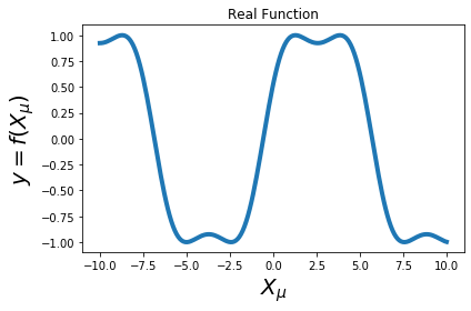
Real Function

Intuition: Confidence Intervals

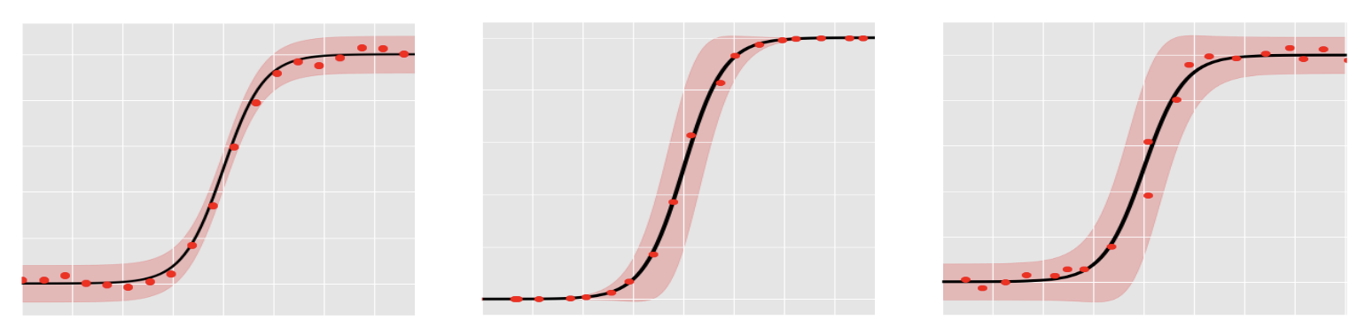Figure: Intuition of for the Taylor expansion for a model:

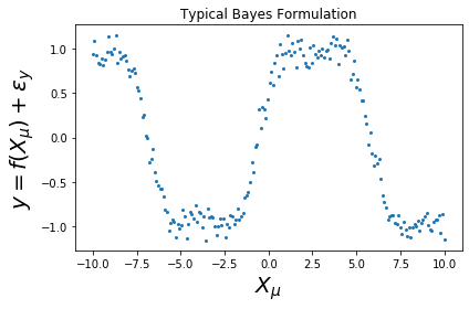
• a) $y=f(\mathbf x) + \epsilon_y$
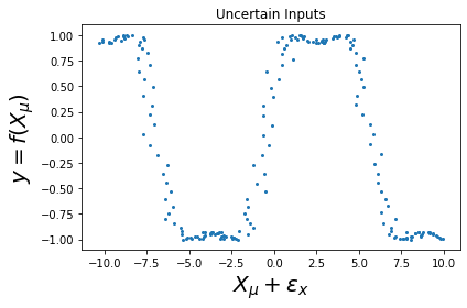
• b) $y=f(\mathbf x + \epsilon_x)$
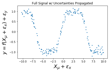
• c) $y=f(\mathbf x + \epsilon_x) + \epsilon_y$

The key idea to think about is what contributes to how far away the error bars are from the approximated mean function. The above graphs will help facilitate the argument given below. There are two main components:

1. Output noise $\epsilon_y$ - the further away the output points are from the approximated function will contribute to the confidence intervals. However, this will affect the vertical components where it is flat and not so much when there is a large slope.
2. Input noise $\epsilon_x$ - the influence of the input noise depends on the slope of the function. i.e. if the function is fully flat, then the input noise doesn't affect the vertical distance between our measurement point and the approximated function; contrast this with a function fully sloped then we have a high contribution to the confidence interval.

So there are two components of competing forces: $\sigma_y^2$ and $\epsilon_x$ and the $\epsilon_x$ is dependent upon the slope of our function $\partial f(\cdot)$ w.r.t. $\mathbf x$.

Epistemic Uncertainty, $\nu_{**}^2$

The second term is the uncertainty over the function values before the noise corruption $\sigma^2$. In this instance, we find

---

Uncertainty in the Error Generalization

First we would like to define all of the sources of uncertainty more concretely. Let's say we have a model $y=f(x)+e$. For starters, we can decompose the generalization error term:

$$\mathcal{E}(\hat{f}) = \mathbb{E}\left[ l(f(x) + e, \hat{f}(x)) \right]$$

$$\mathcal{E}(\hat{f}) = \mathcal{E}(f) + \left( \mathcal{E}(\hat{f}) - \mathcal{E}(f^*) \right) + \left( \mathcal{E}(f^*) - \mathcal{E}(f) \right)$$

$$\mathcal{E}(\hat{f}) = \underset{\text{Bayes Rate}}{\mathcal{E}_{y}} + \underset{\text{Estimation}}{\mathcal{E}_{x}} + \underset{\text{Approx. Error}}{\mathcal{E}_{f}}$$

where $\mathcal{E}_{y}$ is the best possible prediction we can achieve do to the noise $e$ thus it cannot be avoided; $\mathcal{E}_{x}$ is due to the finite-sample problem; and $\mathcal{E}_{f}$ is the model 'wrongness' (the fact that all models are wrong but some are useful). \textbf{Note:} as the number of samples decrease, then the model wrongness will increase. More samples will also allow us to decrease the estimation error. However, many times we are still certain of our uncertainty and we would like to propagate this knowledge through our ML model.

Uncertainty Over Functions

In this section, we will look at the Bayesian treatment of uncertainty and will continue to define the terms aleatoric and epistemic uncertainty in the Bayesian language. Below we briefly outline the Bayesian model functionality in terms of Neural networks.

Prior:

$$p(w_{h,d}) = \mathcal{N}(w_{h,d} | 0, s^2)$$

where $W \in \mathbb{R}^{H \times D}$.

Likelihood

$$p(Y|X, W) = \prod_H \mathcal{N}(y_h | f^W(x_h), \sigma^2)$$

where $f^W(x) = W^T\phi(x)$, $\phi(x)$ is a N dimensional vector.

Posterior

$$P(W|X,Y) = \mathcal{N}(W| \mu, \Sigma)$$

where:

• $\mu = \Sigma \sigma^{-2}\Phi(X)^TY$
• $\Sigma = (\sigma^{-2} \Phi(X)^\top\Phi(X) + s^2\mathbf{I}_D)^{-1}$

Predictive

$$p(y^*|x^*, X, Y) = \mathcal{N}(y^*| \mu_*, \nu_{**}^2)$$

where:

• $\mu_* = \mu^T\phi(X^*)$
• $\nu_{**}^2 = \sigma^2 + \phi(x^*)^\top\Sigma \phi(x^*)$

Strictly speaking from the predictive uncertainty formulation above, uncertainty has two components: the variance from the likelihood term $\sigma^2$ and the variance from the posterior term $\nu_{**}^2$.

---

Distribution Shift

In ML, we typically assume that our data is stationary; meaning that it will always come from the same distribution. This is not always the case as sometimes we just only observed a portion of the data, e.g. space and time.

Need Example: Earth science, in time and space?

This is also essential in the causality realm where such a bad assumption could lead to incorrect causal graphs.