TF2.X and PyTorch¶

For not so Dummies

J. Emmanuel Johnson

What is Deep Learning?¶

Deep Learning is a methodology: building a model by assembling parameterized modules into (possibly dynamic) graphs and optimizing it with gradient-based methods. - Yann LeCun

Deep Learning is a collection of tools to build complex modular differentiable functions. - Danilo Rezende

It's more or less a tool...¶

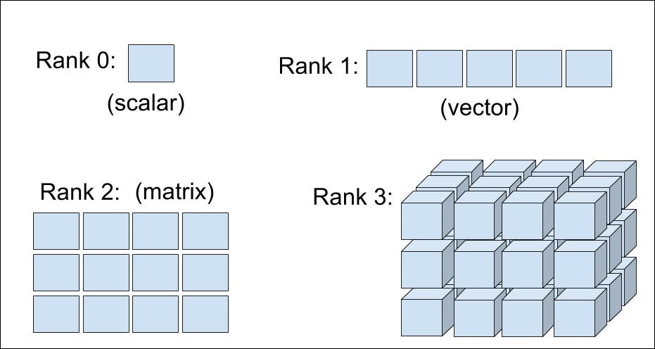
Tensor structures
Automatic differentiation (AutoGrad)
Model Framework (Layers, etc)
Optimizers
Loss Functions

Software Perspective¶

Who is your audience?
What's your scope?
Modular design
Influencing minds...

drawing

User 1¶

My employer gave me some data of landmass in Africa and wants me to find some huts. He thinks Deep Learning can help.

User 2¶

I think I would like one network for my $X$ and $y$ . I also think maybe I should have another network with shared weights and a latent space. Maybe I coud also have two or three input locations. In addition...

User 3¶

I want to implement a Neural Network with convolutional layers and a noise contrastive prior. The weights of the network will be parameterized by Normal distributions. I would also like a training scheme with a mixture of Importance sampling and variational inference with a custom KLD loss.

One Deep Learning library to rule them all...!

Probably a bad idea...

Deep Learning Library Gold Rush¶

Currently more than 10+ mainstream libraries
All tech companies want a piece

Growth of PyTorch¶

drawing

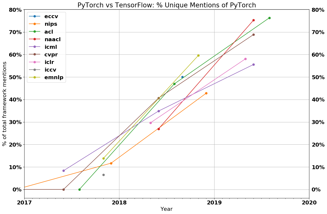
Why?¶

Simple (Pythonic)
Great API
Performance vs Productivity Tradeoff
Easy to Install...

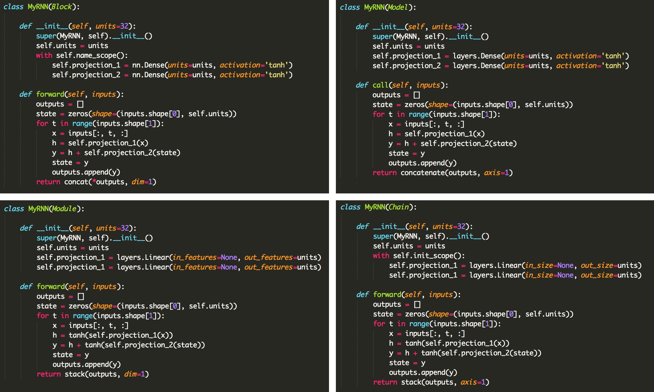
Game: Which Library?¶

drawing

My Suggestions¶

Productivity: Fastai
From Scratch: JAX
Research: PyTorch
Production/Industry: TensorFlow

Basics¶

Tensors
Variables
Automatic differentiation (AutoGrad)

Tensors¶

drawing

Constants¶

# create constant
x = tf.constant([[5, 2], [1, 3]])
print(x)

tf.Tensor(
[[5 2]
 [1 3]], shape=(2, 2), dtype=int32)

¶

Standard¶

# create ones tensor
t_ones = tf.ones(shape=(2, 1))

# create zeros tensor
t_zeros = tf.zeros(shape=(2, 1))

¶

Standard Randomized¶

# pretty standard
tf.random.normal(shape=(2, 2), mean=0., stddev=1.)

# pretty much the same
tf.random.uniform(shape=(2, 2), minval=0, maxval=10)

Variables¶

# set initial value
initial_value = tf.random.normal(shape=(2, 2))

# set variable
a = tf.Variable(initial_value)

Options (constraint, trainable, shape)
All math operations

Updates¶

# new value
b = tf.random.uniform(shape=(2, 2))

# set value
a.assign(b)

# increment (a + b)
a.assign_add(b)

# dencrement (a - b)
a.assign_sub(new_a)

Gradients¶

Gradient Function¶

# init variable
a = tf.Variable(init_value)
# do operation
c = tf.sqrt(tf.square(a) + tf.square(b))
# calculate gradient ( dc/da )
dc_da = tf.gradients(c, a)
# calculate multiple gradients
dc_da, dc_db = tf.gradients(c, [a, b])

New: GradientTape
Defines the scope
literally "record operations"

# init variable
a = tf.Variable(init_value)

# define gradient scope
with tf.GradientTape() as tape:
    # do operation
    c = tf.sqrt(tf.square(a) + tf.square(b))
    # extract gradients ( dc/da )
    dc_da = tape.gradient(c, a)

Nested Gradients¶

# init variable
a = tf.Variable(init_value)

# define gradient scope
with tf.GradientTape() as outer_tape:
    with tf.GradientTape() as inner_tape:
        # do operation
        c = tf.sqrt(tf.square(a) + tf.square(b))
        # extract gradients ( dc/da )
        dc_da = tape.gradient(c, a)
    # extract gradients ( d2c/da2 )
    d2c_da2 = outer_tape.gradient(dc_da, a)

Gradients in PyTorch¶

Same gradient function torch.autograd.grad
There is no Tape
Each variable has their own gradient

# init variable
a = torch.tensor(init_value, requires_grad=True)
# do operation
c = math.sqrt(a ** 2 + b ** 2)
# calculate gradients ( dc/da )
c.backward(a)
# extract gradients
dc_da = a.grad

TF: Engine Module¶

Layer
Network - DAG graph
Model
Sequential

Various Subclasses¶

Layers
Metric
Loss
Callbacks
Optimizer
Regularizers, Constraints

`Layer` Class¶

The core abstraction
Everything is a Layer
...or interacts with a layer

Example Layer¶

$y = \mathbf{W}x + b$

# Subclass Layer
class Linear(tf.keras.Layer):
    def __init__(self):
        super().__init__()
        # Make Parameters

    def call(self, inputs):
        # Do stuff
        return inputs

1 - Constructor¶

# Inherit Layer class
class Linear(tf.keras.Layer):
    def __init__(self, units=32, input_dim=32):
        super().__init__()

2 - Parameters, $\mathbf{W}$ ¶

        # initialize weights (random)
        w_init = tf.random_normal_initializer()(
            shape=(input_dim, units)
        )
        # weights parameter
        self.w = tf.Variable(
            initial_value=w_init,
            trainable=True
        )

2 - Parameter, $b$ ¶

        # initialize bias (zero)
        b_init = tf.zeros_initializer()(
            shape=(units,)
        )
        # bias parameter
        self.b = tf.Variable(
            initial_value=b_init,
            trainable=True
        )

3 - Call Function, $\mathbf{W}x +b$ ¶

    def call(self, inputs):
        return tf.matmul(inputs, self.w) + b

class Linear(tf.keras.Layer):
    def __init__(self, units=32, input_dim=32):
        super().__init__()
        w_init = tf.random_normal_initializer()(
            shape=(input_dim, units)
        )
        # weights parameter
        self.w = tf.Variable(
            initial_value=w_init,
            trainable=True
        )
        # initialize bias (zero)
        b_init = tf.zeros_initializer()(
            shape=(units,)
        )
        # bias parameter
        self.b = tf.Variable(
            initial_value=b_init,
            trainable=True
        )
    def call(self, inputs):
        return tf.matmul(inputs, self.w) + b

PyTorch (the same...)¶

class Linear(nn.Module):
    def __init__(self, units: int, input_dim: int):
        super().__init__()
        # weight 'matrix'
        self.weights = nn.Parameter(
            torch.randn(input_dim, units) / math.sqrt(input_dim),
            requires_grad=True
        )
        # bias vector
        self.bias = nn.Parameter(
            torch.zeros(units),
            requires_grad=True
        )

    def forward(self, inputs):
        return inputs @ self.weights + self.bias

Using it¶

# data
x_train = ...

# initialize linear layer
linear_layer = Linear(units=4, input_dim=2)

# same thing as linear_layer.call(x)
y = linear_layer(x)

TensorFlow `build`¶

Know the # of nodes
Don't know the input shape
More conventional

For example...

    def build(self, input_shape):
        # Weights variable
        self.w = self.add_weight(
            shape=(input_shape[-1], self.units), 
            initializer='random_normal',
            trainable=True
        )
        # Bias variable
        self.b = self.add_weight(
            shape=(self.units,),
            initializer='zeros',
            trainable=True
        )

More convenient...

# data
x_train = ...

# initialize linear layer (without input dims)
linear_layer = Linear(units=4)

# internally -> calls x.shape
y = linear_layer(x)

We can nest as many Layers as we want.

Linear¶

class Linear(Layer):
    def __init__(self, units=32):
        super().__init__()
        # call linear layer
        self.linear = Linear(units)

    def call(self, inputs):
        x = self.linear(inputs)
        return x

Linear Block¶

class LinearBlock(Layer):
    def __init__(self):
        super().__init__()
        self.lin_1 = Linear(32)
        self.lin_2 = Linear(32)
        self.lin_3 = Linear(1)

    def call(self, inputs):
        x = self.lin_1(x)
        x = self.lin_2(x)
        x = self.lin_3(x)
        return x

Training TF2.X, PyTorch¶

Losses¶

TensorFlow

# example loss function 
loss_func = torch.nn.MSELoss()

PyTorch

# example loss function
loss_fn = tf.keras.losses.MSELoss()

Optimizers¶

TensorFlow

# example optimizer
optimizer = tf.keras.optimizers.Adam()

PyTorch

# example optimizer
optimizer = optim.SGD(model.parameters(), lr=0.01)

Full Training Loop (PyTorch)¶

# Loop through batches
for x, y in dataset:
    # initialize gradients
    optimizer.zero_grad()
    # predictions for minibatch
    ypred = lr_model(xbatch)
    # loss value for minibatch
    loss = loss_func(ypred, ybatch)
    # find gradients
    loss.backward()
    # apply optimization
    optimizer.step()

Full Training Loop (TF2.X)¶

for x, y in dataset:
    with tf.GradientTape() as tape:
        # predictions for minibatch
        preds = model(x)
        # loss value for minibatch
        loss = loss_fn(y, preds)
    # find gradients
    grads = tape.gradients(loss, model.trainable_weights)
    # apply optimization
    optimizer.apply_gradients(zip(grads, model.trainable_weights))

TensorFlow Nuggets¶

Training Call¶

Allows training versus inference mode
Just need an extra argument training=True in the call method
Prob Models, e.g. Batch Norm., Variational Inference

Example¶

...
def call(self, x, training=True):
    if training:
        # do training stuff
    else:
        # do inference stuff
    return x

Add Loss¶

"Add Losses on the fly"
Each layer has it's own regularization
Examples: KLD, Activation or Weight Regularization

Example - Model¶

class MLP(Layer):
    def __init__(self, units=32, reg=1e-3):
        super().__init__()
        self.linear = Linear(units)
        self.reg = reg
    def call(self, inputs):
        x = self.linear(inputs)
        x = tf.nn.relu(x)
        # Add loss during the call
        self.add_loss(tf.reduce_sum(output ** 2) * self.reg)
        return x

¶

Example - Training¶

mlp_model = MLP(32)                 # initialize model
loss_fn = tf.keras.losses.MSELoss() # loss function
opt = tf.keras.optimizers.Adam()    # optimizer
# Loop through dataset
for x, y in dataset:
    with tf.GradientTape() as tape:
        preds = mlp_model(x)            # predictions
        loss = loss_fn(y, preds)        # loss value
        loss += sum(mlp_model.losses)   # extra losses
    # find gradients
    grads = tape.gradients(loss, model.trainable_weights)
    # apply optimization
    opt.apply_gradients(zip(grads, model.trainable_weights))

Compile Code¶

Use a decorator, @tf.function
Optional
Easy performance booster

Example - Graphs¶

@tf.function
def train_step(dataset):
    for x, y in dataset:
        with tf.GradientTape() as tape:
            preds = mlp_model(x)            # predictions
            loss = loss_fn(y, preds)        # loss value
            loss += sum(mlp_model.losses)   # extra losses
        # find gradients
        grads = tape.gradients(loss, model.trainable_weights)
        # apply optimization
        opt.apply_gradients(zip(grads, model.trainable_weights))
        return loss

Model Class¶

Can do everything a Layer can do
Built-in functionality
a.k.a. Keras territory
TF and PyTorch part ways

Definitions¶

Layer:

A closed sequence of operation
e.g. convolutional layer, recurrent layer, resnet block, attention block.

Model:

The top layer of your algorithm
e.g. Deep learning model, deep neural network.

Training Functionality¶

.compile()
.fit()
.evaulate()
.predict()
.save()
.summary()
.plot_model()

Example -¶

# loss function
loss = tf.keras.losses.MSELoss(from_logits=True)
# accuracy metrics
accuracy = tf.keras.metrics.SparseCategoricalAccuracy()
# optimizer
optimizer = tf.keras.optimizers.Adam()
# compile to graph
model.compile(optimizer=optimizer, loss=loss, metrics=[accuracy])
# Fit Model
model.fit(dataset, epochs=3)
# Test Data
loss, acc = model.evaluate(test_dataset)

Functional Models¶

Creates DAG
Model Class with Extras
Only in TF

drawing

Simple Example¶

# input checks
x = tf.keras.layers.Flatten(shape=28, 28))(inputs)
# Layer 1
x = tf.keras.layers.Dense(512, activation=tf.nn.relu)(inputs)
# Layer 2
x = tf.keras.layers.Dropout(0.2)(x)
# outputs
x = tf.keras.layers.Dense(10, activation=tf.nn.softmax)(x)
# create model class
model = tf.keras.Model(inputs, outputs)
# compile
model.compile(
    optimizer='adam', 
    loss='sparse_categorical_crossentropy',
    metrics=['accuracy']
)

Example - Graph Output¶

drawing

We can go crazy...¶

drawing

Sequential Models¶

Predifined
PyTorch & TF
In TF, Model class

PyTorch

model = nn.Sequential(
  torch.nn.Linear(256),
  F.reLU(),
  torch.nn.Linear(256),
  F.reLU(),
  torch.nn.Linear(10),
)

TensorFlow

model = tf.keras.Sequential([
  layers.Dense(256, activation=tf.nn.relu),
  layers.Dense(256, activation=tf.nn.relu),
  layers.Dense(10)
])

Datasets¶

Convenience Functions
Take care of loading, iterations, batches

Normally¶

n_batches = (n_samples - 1) // batch_size + 1

for idx in range(n_batches):
    # get indices for batches
    start_idx = idx * batch_size
    end_idx   = start_idx + batch_size
    # get subset from data
    xbatch = x_train[start_idx:end_idx]
    ybatch = y_train[start_idx:end_idx]

PyTorch - Datasets¶

# create dataset
train_ds = TensorDataset(x_train, y_train)
# Loop through batches
    for start_idx, end_idx in range(batch_idx):
        # Use Dataset to store training data
        xbatch, ybatch = train_ds[start_idx:end_idx]
        # Do stuff...

Note: In PyTorch, the Dataset helps us to do index and slice through our data. It also can combine inputs and outputs so that we only have to slice through a single dataset. It can even convert your np.ndarray dataset to a Tensor automatically.

PyTorch - DataLoaders¶

# create dataset
train_ds = TensorDataset(x_train, y_train)
# create dataloader
train_dl = DataLoader(train_ds, batch_size=100)
# Loop through batches
    for xbatch, ybatch in train_dl:
        # Do stuff...

TF - Both...¶

# create dataset
train_ds = tf.data.Dataset.from_tensor_slices(
    (x_train, y_train)
)
# create dataloader
train_dl = train_ds.batch(100)
# Loop through batches
    for xbatch, ybatch in train_dl:
        # Do stuff...

What We Covered¶

DL Framework Idea
Layers and Models
Sequential Model

What We didn't Cover¶

Callbacks
Distributed Training
Multiple GPUs
All options under the sun
Tensorboard (Built-in Jupyter Notebooks!)

Summary¶

drawing

TensorFlow Training¶

drawing

TF2.X and PyTorch¶

What is Deep Learning?¶

It's more or less a tool...¶

Software Perspective¶

User 1¶

User 2¶

User 3¶

Deep Learning Library Gold Rush¶

Growth of PyTorch¶

Why?¶

Game: Which Library?¶

My Suggestions¶

Basics¶

Tensors¶

Constants¶

tf.Tensor( [[5 2] [1 3]], shape=(2, 2), dtype=int32) ¶

Standard¶

# create ones tensor t_ones = tf.ones(shape=(2, 1)) # create zeros tensor t_zeros = tf.zeros(shape=(2, 1)) ¶

Standard Randomized¶

Variables¶

Updates¶

Gradients¶

Gradient Function¶

Nested Gradients¶

Gradients in PyTorch¶

TF: Engine Module¶

Various Subclasses¶

Layer Class¶

Example Layer¶

1 - Constructor¶

2 - Parameters, \mathbf{W}\mathbf{W}¶

2 - Parameter, bb¶

3 - Call Function, \mathbf{W}x +b\mathbf{W}x +b¶

PyTorch (the same...)¶

Using it¶

TensorFlow build¶

Linear¶

Linear Block¶

Training TF2.X, PyTorch¶

Losses¶

Optimizers¶

Full Training Loop (PyTorch)¶

Full Training Loop (TF2.X)¶

TensorFlow Nuggets¶

Training Call¶

Example¶

Add Loss¶

Example - Model¶

class MLP(Layer): def __init__(self, units=32, reg=1e-3): super().__init__() self.linear = Linear(units) self.reg = reg def call(self, inputs): x = self.linear(inputs) x = tf.nn.relu(x) # Add loss during the call self.add_loss(tf.reduce_sum(output ** 2) * self.reg) return x ¶

Example - Training¶

Compile Code¶

Example - Graphs¶

Model Class¶

Definitions¶

Training Functionality¶

Example -¶

Functional Models¶

Simple Example¶

Example - Graph Output¶

We can go crazy...¶

Sequential Models¶

Datasets¶

Normally¶

PyTorch - Datasets¶

PyTorch - DataLoaders¶

TF - Both...¶

What We Covered¶

What We didn't Cover¶

Summary¶

TensorFlow Training¶

`tf.Tensor( [[5 2] [1 3]], shape=(2, 2), dtype=int32)`
¶

`# create ones tensor t_ones = tf.ones(shape=(2, 1)) # create zeros tensor t_zeros = tf.zeros(shape=(2, 1))`
¶

`Layer` Class¶

2 - Parameters, $\mathbf{W}$ ¶

2 - Parameter, $b$ ¶

3 - Call Function, $\mathbf{W}x +b$ ¶

TensorFlow `build`¶

`class MLP(Layer): def init(self, units=32, reg=1e-3): super().init() self.linear = Linear(units) self.reg = reg def call(self, inputs): x = self.linear(inputs) x = tf.nn.relu(x) # Add loss during the call self.add_loss(tf.reduce_sum(output ** 2) * self.reg) return x`
¶