MCMC eGP
TLDR
I did a quick experiment where I look at how we can impact the error bars when doing a fully Bayesian GP (i.e. GP with MCMC inference). I have 3 cases where I use no prior on the inputs, where I use a modest prior on the inputs, and one where I use the exact known prior on the inputs. The results are definitely different than what I'm used to because I actually trained the GP knowing the priors. The error bars were reduced which I guess makes sense.
TODO: Do the MCMC where we approximate the posterior when we trained the GP with uncertain inputs.
Experiment
Code Blocks
!pip install jax jaxlib numpyro
Requirement already satisfied: jax in /usr/local/lib/python3.6/dist-packages (0.1.62)
Requirement already satisfied: jaxlib in /usr/local/lib/python3.6/dist-packages (0.1.42)
Collecting numpyro
[?25l Downloading https://files.pythonhosted.org/packages/b8/58/54e914bb6d8ee9196f8dbf28b81057fea81871fc171dbee03b790336d0c5/numpyro-0.2.4-py3-none-any.whl (159kB)
[K |████████████████████████████████| 163kB 2.5MB/s
[?25hRequirement already satisfied: absl-py in /usr/local/lib/python3.6/dist-packages (from jax) (0.9.0)
Requirement already satisfied: opt-einsum in /usr/local/lib/python3.6/dist-packages (from jax) (3.2.1)
Requirement already satisfied: numpy>=1.12 in /usr/local/lib/python3.6/dist-packages (from jax) (1.18.3)
Requirement already satisfied: scipy in /usr/local/lib/python3.6/dist-packages (from jaxlib) (1.4.1)
Requirement already satisfied: tqdm in /usr/local/lib/python3.6/dist-packages (from numpyro) (4.38.0)
Requirement already satisfied: six in /usr/local/lib/python3.6/dist-packages (from absl-py->jax) (1.12.0)
[31mERROR: numpyro 0.2.4 has requirement jax==0.1.57, but you'll have jax 0.1.62 which is incompatible.[0m
[31mERROR: numpyro 0.2.4 has requirement jaxlib==0.1.37, but you'll have jaxlib 0.1.42 which is incompatible.[0m
Installing collected packages: numpyro
Successfully installed numpyro-0.2.4
#@title packages

import time

import numpy as onp
from dataclasses import dataclass

import jax
from jax import vmap
import jax.numpy as np
import jax.random as random

import numpyro
import numpyro.distributions as dist
from numpyro.infer import MCMC, NUTS

import matplotlib
import matplotlib.pyplot as plt
import seaborn as sns

sns.reset_defaults()
#sns.set_style('whitegrid')
#sns.set_context('talk')
sns.set_context(context='talk',font_scale=0.7)
%matplotlib inline
#@title Data

def get_data(N=30, sigma_inputs=0.15, sigma_obs=0.15, N_test=400):
    onp.random.seed(0)
    X = np.linspace(-10, 10, N)
    # Y = X + 0.2 * np.power(X, 3.0) + 0.5 * np.power(0.5 + X, 2.0) * np.sin(4.0 * X)
    Y = np.sin(1.0 * np.pi / 1.6 * np.cos(5 + .5 * X))
    Y += sigma_obs * onp.random.randn(N)
    X += sigma_inputs * onp.random.randn(N)
    Y -= np.mean(Y)
    Y /= np.std(Y)

    assert X.shape == (N,)
    assert Y.shape == (N,)

    X_test = np.linspace(-11, 11, N_test)
    X_test += sigma_inputs * onp.random.randn(N_test)

    return X, Y, X_test
GP Model
#@title GP Model

# squared exponential kernel with diagonal noise term
def kernel(X, Z, var, length, noise, jitter=1.0e-6, include_noise=True):
    deltaXsq = np.power((X[:, None] - Z) / length, 2.0)
    k = var * np.exp(-0.5 * deltaXsq)
    if include_noise:
        k += (noise + jitter) * np.eye(X.shape[0])
    return k

def model(Xmu, Y):
    # set uninformative log-normal priors on our three kernel hyperparameters
    var = numpyro.sample("kernel_var", dist.LogNormal(0.0, 10.0))
    noise = numpyro.sample("kernel_noise", dist.LogNormal(0.0, 10.0))
    length = numpyro.sample("kernel_length", dist.LogNormal(0.0, 10.0))
    # X = numpyro.sample("X", dist.Normal(Xmu, 0.15 * np.ones((Xmu.shape[0],))))
    X = Xmu

    # compute kernel
    k = kernel(X, X, var, length, noise)

    # sample Y according to the standard gaussian process formula
    numpyro.sample("Y", dist.MultivariateNormal(loc=np.zeros(X.shape[0]), covariance_matrix=k),
                   obs=Y)
# helper function for doing hmc inference
def run_inference(model, args, rng_key, X, Y):
    start = time.time()
    kernel = NUTS(model)
    mcmc = MCMC(kernel, args.num_warmup, args.num_samples, num_chains=args.num_chains,
                progress_bar=True)
    mcmc.run(rng_key, X, Y)
    mcmc.print_summary()
    print('\nMCMC elapsed time:', time.time() - start)
    return mcmc.get_samples()


# do GP prediction for a given set of hyperparameters. this makes use of the well-known
# formula for gaussian process predictions
def predict(rng_key, X, Y, X_test, var, length, noise):
    # compute kernels between train and test data, etc.
    k_pp = kernel(X_test, X_test, var, length, noise, include_noise=True)
    k_pX = kernel(X_test, X, var, length, noise, include_noise=False)
    k_XX = kernel(X, X, var, length, noise, include_noise=True)
    K_xx_inv = np.linalg.inv(k_XX)
    K = k_pp - np.matmul(k_pX, np.matmul(K_xx_inv, np.transpose(k_pX)))
    sigma_noise = np.sqrt(np.clip(np.diag(K), a_min=0.)) * jax.random.normal(rng_key, X_test.shape[:1])
    mean = np.matmul(k_pX, np.matmul(K_xx_inv, Y))
    # we return both the mean function and a sample from the posterior predictive for the
    # given set of hyperparameters
    return mean, mean + sigma_noise
Experiment
@dataclass
class args:
    num_data = 60
    num_warmup = 100
    num_chains = 1
    num_samples = 1_000
    device = 'cpu'
    sigma_inputs = 0.3
    sigma_obs = 0.05

numpyro.set_platform(args.device)
X, Y, X_test = get_data(args.num_data, sigma_inputs=args.sigma_inputs, sigma_obs=args.sigma_obs)
rng_key, rng_key_predict = random.split(random.PRNGKey(0))

# Run inference scheme
samples = run_inference(model, args, rng_key, X, Y, )
sample: 100%|██████████| 1100/1100 [00:11<00:00, 96.81it/s, 7 steps of size 6.48e-01. acc. prob=0.94]


                     mean       std    median      5.0%     95.0%     n_eff     r_hat
  kernel_length      1.97      0.23      1.97      1.58      2.34    650.87      1.00
   kernel_noise      0.04      0.01      0.04      0.02      0.05    637.46      1.00
     kernel_var      1.15      0.65      0.98      0.34      1.97    563.69      1.00

Number of divergences: 0

MCMC elapsed time: 14.073462963104248
Predictions
# do prediction
vmap_args = (random.split(rng_key_predict, args.num_samples * args.num_chains), samples['kernel_var'],
                samples['kernel_length'], samples['kernel_noise'])
means, predictions = vmap(lambda rng_key, var, length, noise:
                            predict(rng_key, X, Y, X_test, var, length, noise))(*vmap_args)

mean_prediction = onp.mean(means, axis=0)
percentiles = onp.percentile(predictions, [5.0, 95.0], axis=0)
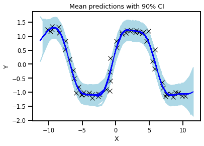
# make plots
fig, ax = plt.subplots(1, 1)

# plot training data
ax.plot(X, Y, 'kx')
# plot 90% confidence level of predictions
ax.fill_between(X_test, percentiles[0, :], percentiles[1, :], color='lightblue')
# plot mean prediction
ax.plot(X_test, mean_prediction, 'blue', ls='solid', lw=2.0)
ax.set(xlabel="X", ylabel="Y", title="Mean predictions with 90% CI")
[Text(0, 0.5, 'Y'),
 Text(0.5, 0, 'X'),
 Text(0.5, 1.0, 'Mean predictions with 90% CI')]
GP Model - Uncertain Inputs
def emodel(Xmu, Y):
    # set uninformative log-normal priors on our three kernel hyperparameters
    var = numpyro.sample("kernel_var", dist.LogNormal(0.0, 10.0))
    noise = numpyro.sample("kernel_noise", dist.LogNormal(0.0, 10.0))
    length = numpyro.sample("kernel_length", dist.LogNormal(0.0, 10.0))
    X = numpyro.sample("X", dist.Normal(Xmu, 0.3), )
    # X = Xmu + Xstd
    # X = numpyro.sample("X", dist.Normal(Xmu, 0.3 * np.ones(Xmu.shape[-1])), )


    # compute kernel
    k = kernel(X, X, var, length, noise)

    # sample Y according to the standard gaussian process formula
    numpyro.sample("Y", dist.MultivariateNormal(loc=np.zeros(X.shape[0]), covariance_matrix=k),
                   obs=Y)
rng_key, rng_key_predict = random.split(random.PRNGKey(0))

# Run inference scheme
samples = run_inference(emodel, args, rng_key, X, Y, )
sample: 100%|██████████| 1100/1100 [00:19<00:00, 56.73it/s, 15 steps of size 2.14e-01. acc. prob=0.93]


                     mean       std    median      5.0%     95.0%     n_eff     r_hat
           X[0]    -10.01      0.25     -9.98    -10.40     -9.59    597.56      1.00
           X[1]     -9.91      0.27     -9.92    -10.30     -9.45    887.43      1.00
           X[2]     -9.65      0.27     -9.67    -10.03     -9.16    475.77      1.00
           X[3]     -9.40      0.25     -9.41     -9.85     -9.04    937.07      1.00
           X[4]     -8.83      0.23     -8.83     -9.27     -8.51    759.05      1.00
           X[5]     -8.33      0.19     -8.31     -8.61     -8.01    463.77      1.00
           X[6]     -8.31      0.19     -8.30     -8.60     -8.01    556.40      1.00
           X[7]     -7.77      0.13     -7.77     -7.98     -7.57    554.29      1.00
           X[8]     -7.42      0.12     -7.42     -7.62     -7.23    426.67      1.00
           X[9]     -7.03      0.11     -7.03     -7.21     -6.84    363.45      1.00
          X[10]     -6.60      0.12     -6.61     -6.79     -6.41    370.03      1.00
          X[11]     -6.29      0.13     -6.29     -6.51     -6.10    423.12      1.00
          X[12]     -5.80      0.16     -5.80     -6.05     -5.54    461.56      1.00
          X[13]     -5.45      0.18     -5.46     -5.74     -5.15    665.71      1.00
          X[14]     -5.00      0.25     -5.02     -5.41     -4.61   1038.74      1.00
          X[15]     -4.97      0.23     -4.98     -5.32     -4.59    782.89      1.00
          X[16]     -4.92      0.32     -4.93     -5.42     -4.40   1370.20      1.00
          X[17]     -4.41      0.29     -4.41     -4.87     -3.91   1293.31      1.00
          X[18]     -4.00      0.31     -3.99     -4.49     -3.50   1020.15      1.00
          X[19]     -3.57      0.28     -3.55     -4.06     -3.14    686.66      1.00
          X[20]     -3.42      0.36     -3.40     -3.96     -2.79    798.33      1.00
          X[21]     -2.57      0.36     -2.57     -3.12     -1.96    760.66      1.00
          X[22]     -2.34      0.28     -2.32     -2.82     -1.92    800.18      1.00
          X[23]     -2.68      0.27     -2.66     -3.07     -2.18    779.41      1.00
          X[24]     -1.61      0.16     -1.61     -1.89     -1.38    410.05      1.01
          X[25]     -1.65      0.16     -1.65     -1.91     -1.38    460.06      1.00
          X[26]     -1.16      0.13     -1.16     -1.36     -0.96    352.57      1.01
          X[27]     -0.81      0.12     -0.80     -0.98     -0.59    363.98      1.01
          X[28]     -0.32      0.12     -0.33     -0.51     -0.13    388.07      1.01
          X[29]      0.11      0.12      0.10     -0.10      0.29    393.42      1.02
          X[30]      0.41      0.13      0.40      0.18      0.62    534.79      1.01
          X[31]      0.93      0.19      0.92      0.63      1.24    897.67      1.00
          X[32]      1.08      0.21      1.07      0.75      1.42    398.94      1.00
          X[33]      1.39      0.33      1.36      0.87      1.90    443.17      1.00
          X[34]      1.67      0.28      1.67      1.25      2.13    822.54      1.00
          X[35]      2.07      0.30      2.07      1.60      2.55    735.84      1.00
          X[36]      2.18      0.30      2.18      1.69      2.65    546.85      1.00
          X[37]      3.10      0.31      3.10      2.63      3.64   1153.64      1.00
          X[38]      2.92      0.28      2.93      2.46      3.35   1498.27      1.00
          X[39]      3.33      0.30      3.34      2.82      3.79   1393.60      1.00
          X[40]      4.02      0.26      4.03      3.64      4.48    743.00      1.00
          X[41]      3.50      0.31      3.50      3.01      3.99    895.25      1.00
          X[42]      3.93      0.33      3.96      3.41      4.47    667.17      1.00
          X[43]      4.27      0.19      4.27      3.96      4.60    626.95      1.00
          X[44]      4.89      0.16      4.88      4.62      5.14    340.23      1.00
          X[45]      5.36      0.13      5.36      5.17      5.58    373.83      1.00
          X[46]      5.78      0.12      5.78      5.58      5.96    307.39      1.00
          X[47]      6.05      0.12      6.06      5.86      6.24    329.60      1.00
          X[48]      6.65      0.13      6.64      6.45      6.86    343.38      1.00
          X[49]      6.94      0.15      6.94      6.68      7.18    385.53      1.00
          X[50]      7.56      0.26      7.53      7.18      8.04    551.86      1.00
          X[51]      7.61      0.26      7.59      7.17      8.03    524.45      1.00
          X[52]      7.63      0.21      7.63      7.25      7.95   1001.54      1.00
          X[53]      8.40      0.30      8.38      7.91      8.89    576.53      1.00
          X[54]      8.28      0.33      8.32      7.69      8.78   1210.06      1.00
          X[55]      8.95      0.26      8.95      8.50      9.34   1332.43      1.00
          X[56]      9.25      0.27      9.25      8.77      9.65   1931.84      1.00
          X[57]      9.27      0.27      9.28      8.82      9.69   1255.06      1.00
          X[58]      9.89      0.28      9.91      9.46     10.36    613.94      1.00
          X[59]     10.22      0.28     10.20      9.78     10.66    925.47      1.00
  kernel_length      1.95      0.19      1.96      1.63      2.23    440.62      1.01
   kernel_noise      0.00      0.00      0.00      0.00      0.01    222.75      1.00
     kernel_var      1.18      0.64      1.02      0.39      2.01    423.49      1.01

Number of divergences: 0

MCMC elapsed time: 23.19466996192932
# do prediction
vmap_args = (random.split(rng_key_predict, args.num_samples * args.num_chains), samples['kernel_var'],
                samples['kernel_length'], samples['kernel_noise'])
means, predictions = vmap(lambda rng_key, var, length, noise:
                            predict(rng_key, X, Y, X_test, var, length, noise))(*vmap_args)

mean_prediction = onp.mean(means, axis=0)
percentiles = onp.percentile(predictions, [5.0, 95.0], axis=0)
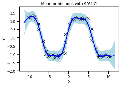
# make plots
fig, ax = plt.subplots(1, 1)

# plot training data
ax.plot(X, Y, 'kx')
# plot 90% confidence level of predictions
ax.fill_between(X_test, percentiles[0, :], percentiles[1, :], color='lightblue')
# plot mean prediction
ax.plot(X_test, mean_prediction, 'blue', ls='solid', lw=2.0)
ax.set(xlabel="X", ylabel="Y", title="Mean predictions with 90% CI")
[Text(0, 0.5, 'Y'),
 Text(0.5, 0, 'X'),
 Text(0.5, 1.0, 'Mean predictions with 90% CI')]
def emodel(Xmu, Y):
    # set uninformative log-normal priors on our three kernel hyperparameters
    var = numpyro.sample("kernel_var", dist.LogNormal(0.0, 10.0))
    noise = numpyro.sample("kernel_noise", dist.LogNormal(0.0, 10.0))
    length = numpyro.sample("kernel_length", dist.LogNormal(0.0, 10.0))
    # X = numpyro.sample("X", dist.Normal(Xmu, 0.15), )
    Xstd = numpyro.sample("Xstd", dist.Normal(0.0, 0.3), sample_shape=(Xmu.shape[0],))
    X = Xmu + Xstd
    # X = numpyro.sample("X", dist.Normal(Xmu, 0.3 * np.ones(Xmu.shape[-1])), )


    # compute kernel
    k = kernel(X, X, var, length, noise)

    # sample Y according to the standard gaussian process formula
    numpyro.sample("Y", dist.MultivariateNormal(loc=np.zeros(X.shape[0]), covariance_matrix=k),
                   obs=Y)
rng_key, rng_key_predict = random.split(random.PRNGKey(0))

# Run inference scheme
samples = run_inference(emodel, args, rng_key, X, Y, )
sample: 100%|██████████| 1100/1100 [00:17<00:00, 62.81it/s, 15 steps of size 2.65e-01. acc. prob=0.89]


                     mean       std    median      5.0%     95.0%     n_eff     r_hat
        Xstd[0]      0.20      0.26      0.22     -0.23      0.62    792.72      1.00
        Xstd[1]     -0.15      0.26     -0.15     -0.63      0.22    951.20      1.00
        Xstd[2]     -0.09      0.26     -0.11     -0.50      0.37    832.81      1.00
        Xstd[3]      0.10      0.24      0.10     -0.28      0.49    982.06      1.00
        Xstd[4]     -0.25      0.22     -0.26     -0.63      0.09    934.13      1.00
        Xstd[5]      0.09      0.19      0.11     -0.19      0.42    531.47      1.00
        Xstd[6]      0.13      0.18      0.15     -0.18      0.43    452.94      1.00
        Xstd[7]     -0.28      0.13     -0.28     -0.49     -0.06    495.33      1.00
        Xstd[8]      0.14      0.13      0.15     -0.05      0.35    365.29      1.00
        Xstd[9]     -0.10      0.12     -0.10     -0.30      0.09    306.55      1.00
       Xstd[10]     -0.21      0.12     -0.20     -0.42     -0.02    304.69      1.00
       Xstd[11]     -0.05      0.13     -0.05     -0.26      0.18    284.53      1.00
       Xstd[12]     -0.21      0.17     -0.21     -0.49      0.05    415.29      1.00
       Xstd[13]      0.52      0.19      0.50      0.20      0.81    540.49      1.00
       Xstd[14]      0.12      0.24      0.11     -0.29      0.47    898.49      1.01
       Xstd[15]      0.15      0.23      0.14     -0.23      0.52   1165.26      1.00
       Xstd[16]     -0.08      0.33     -0.10     -0.60      0.44    904.75      1.00
       Xstd[17]     -0.00      0.29     -0.00     -0.53      0.43   1652.78      1.00
       Xstd[18]     -0.01      0.32      0.00     -0.49      0.54   1462.54      1.00
       Xstd[19]     -0.02      0.28     -0.01     -0.47      0.47    903.68      1.00
       Xstd[20]      0.14      0.36      0.17     -0.47      0.66    905.66      1.00
       Xstd[21]      0.05      0.36      0.06     -0.54      0.61    648.84      1.00
       Xstd[22]      0.04      0.30      0.07     -0.44      0.51   1011.25      1.00
       Xstd[23]     -0.01      0.27      0.00     -0.43      0.45   1237.85      1.00
       Xstd[24]     -0.20      0.16     -0.20     -0.45      0.06    419.10      1.00
       Xstd[25]     -0.69      0.16     -0.68     -0.98     -0.46    379.36      1.00
       Xstd[26]     -0.33      0.13     -0.33     -0.54     -0.12    320.10      1.00
       Xstd[27]      0.09      0.13      0.09     -0.10      0.30    245.93      1.01
       Xstd[28]      0.50      0.13      0.50      0.30      0.71    253.37      1.01
       Xstd[29]     -0.04      0.13     -0.04     -0.24      0.18    259.11      1.01
       Xstd[30]      0.36      0.14      0.36      0.13      0.57    296.81      1.01
       Xstd[31]      0.07      0.19      0.06     -0.23      0.37    539.63      1.00
       Xstd[32]      0.18      0.21      0.17     -0.18      0.50    868.61      1.00
       Xstd[33]     -0.09      0.31     -0.14     -0.54      0.45    551.52      1.00
       Xstd[34]      0.04      0.27      0.04     -0.35      0.53   1343.46      1.00
       Xstd[35]     -0.01      0.29     -0.01     -0.48      0.51   1573.42      1.00
       Xstd[36]     -0.04      0.29     -0.04     -0.51      0.44   1578.87      1.00
       Xstd[37]      0.02      0.31      0.03     -0.48      0.53   2398.18      1.00
       Xstd[38]     -0.00      0.29     -0.00     -0.45      0.47   1411.13      1.00
       Xstd[39]     -0.01      0.30     -0.01     -0.49      0.48   2119.89      1.00
       Xstd[40]     -0.11      0.25     -0.10     -0.49      0.33    537.76      1.00
       Xstd[41]      0.00      0.30      0.01     -0.48      0.51    934.64      1.00
       Xstd[42]      0.09      0.32      0.12     -0.49      0.55   1000.19      1.00
       Xstd[43]     -0.61      0.20     -0.60     -0.92     -0.28    716.21      1.00
       Xstd[44]      0.31      0.15      0.32      0.08      0.57    487.44      1.00
       Xstd[45]     -0.49      0.12     -0.48     -0.68     -0.28    426.20      1.00
       Xstd[46]      0.30      0.12      0.30      0.11      0.49    383.15      1.00
       Xstd[47]      0.34      0.12      0.34      0.15      0.53    329.32      1.00
       Xstd[48]     -0.21      0.13     -0.22     -0.41     -0.01    383.74      1.00
       Xstd[49]     -0.12      0.15     -0.13     -0.37      0.10    392.93      1.00
       Xstd[50]      0.03      0.25      0.01     -0.37      0.40    668.25      1.00
       Xstd[51]      0.05      0.25      0.03     -0.37      0.46    928.56      1.00
       Xstd[52]      0.26      0.22      0.24     -0.12      0.60    776.53      1.00
       Xstd[53]     -0.14      0.33     -0.17     -0.62      0.48    672.39      1.00
       Xstd[54]      0.06      0.32      0.08     -0.49      0.54   1436.10      1.00
       Xstd[55]      0.06      0.26      0.05     -0.35      0.49   1649.02      1.00
       Xstd[56]     -0.02      0.29     -0.02     -0.47      0.44   1683.10      1.00
       Xstd[57]     -0.01      0.27     -0.01     -0.42      0.48   1384.29      1.00
       Xstd[58]      0.05      0.28      0.06     -0.37      0.54   1061.70      1.00
       Xstd[59]     -0.06      0.26     -0.08     -0.46      0.39   1705.82      1.00
  kernel_length      1.93      0.21      1.94      1.57      2.26    224.70      1.01
   kernel_noise      0.00      0.00      0.00      0.00      0.01    262.87      1.00
     kernel_var      1.15      0.62      1.00      0.41      1.95    344.59      1.00

Number of divergences: 0

MCMC elapsed time: 19.7586088180542
# do prediction
vmap_args = (random.split(rng_key_predict, args.num_samples * args.num_chains), samples['kernel_var'],
                samples['kernel_length'], samples['kernel_noise'])
means, predictions = vmap(lambda rng_key, var, length, noise:
                            predict(rng_key, X, Y, X_test, var, length, noise))(*vmap_args)

mean_prediction = onp.mean(means, axis=0)
percentiles = onp.percentile(predictions, [5.0, 95.0], axis=0)
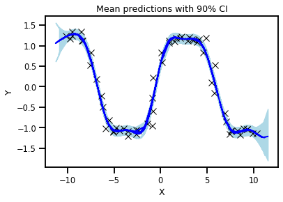
# make plots
fig, ax = plt.subplots(1, 1)

# plot training data
ax.plot(X, Y, 'kx')
# plot 90% confidence level of predictions
ax.fill_between(X_test, percentiles[0, :], percentiles[1, :], color='lightblue')
# plot mean prediction
ax.plot(X_test, mean_prediction, 'blue', ls='solid', lw=2.0)
ax.set(xlabel="X", ylabel="Y", title="Mean predictions with 90% CI")
[Text(0, 0.5, 'Y'),
 Text(0.5, 0, 'X'),
 Text(0.5, 1.0, 'Mean predictions with 90% CI')]
Results