Bayesian updates from scratch — sequential conjugate inference

Notebook 0.4 — three parameterizations showed that combining two Gaussian factors is addition in natural-parameter space. This notebook follows that thread to its conclusion: an inference loop that absorbs $N$ Gaussian observations one at a time, equivalent to processing them all at once, in any order, with the same answer to floating-point precision.

That single idea — exponential-family inference reduces to summing natural parameters — underlies the Kalman filter, GP regression, EP, and most of approximate inference. We make it concrete by

writing the linear-Gaussian Bayes rule once, in natural form, leaning on ((5));
running a sequential loop over $N=6$ noisy observations of an unknown 2D location;
confirming batch = sequential = any-order to $\sim 10^{-15}$ ;
closing with the punch line: GP regression with a Gaussian likelihood is a single application of the same rule.

Prerequisites: 0.2 — MultivariateNormal API, 0.4 — three parameterizations, 0.5 — Joseph-form covariance update.

from __future__ import annotations

import warnings
warnings.filterwarnings("ignore", message=r".*IProgress.*")

import einx
import jax
import jax.numpy as jnp
import lineax as lx
import matplotlib.pyplot as plt
import numpy as np
import gaussx
from gaussx import GaussianExpFam, log_marginal_likelihood, solve, to_expectation, to_natural

jax.config.update("jax_enable_x64", True)
KEY = jax.random.PRNGKey(42)
plt.rcParams.update({
    "figure.dpi": 110,
    "axes.grid": True,
    "axes.grid.which": "both",
    "xtick.minor.visible": True,
    "ytick.minor.visible": True,
    "grid.alpha": 0.3,
})


def psd_op(M):
    return lx.MatrixLinearOperator(M, lx.symmetric_tag)


def ellipse_points(mu, Sigma, n_std=2.0, n=200):
    # Standard 2D confidence-ellipse construction via eigendecomposition.
    theta = jnp.linspace(0.0, 2.0 * jnp.pi, n)
    circle = jnp.stack([jnp.cos(theta), jnp.sin(theta)], axis=0)
    eigvals, eigvecs = jnp.linalg.eigh(Sigma)
    sqrt_l = jnp.sqrt(eigvals) * n_std
    stretched = einx.multiply("j, j t -> j t", sqrt_l, circle)
    rotated   = einx.dot("i j, j t -> i t", eigvecs, stretched)
    return einx.add("i, i t -> i t", mu, rotated)

Linear-Gaussian Bayes rule, in one breath¶

The linear-Gaussian observation model from ((1)) gives a Gaussian posterior with three equivalent updates:

\Lambda_{\rm post} \;=\; \Lambda_{\rm prior} \;+\; H^\top R^{-1} H, \qquad \Lambda_{\rm post}\,\mu_{\rm post} \;=\; \Lambda_{\rm prior}\,\mu_{\rm prior} \;+\; H^\top R^{-1} y.

((1))

In natural parameters, recalling $\eta_1 = \Lambda \mu$ and $\eta_2 = -\tfrac12 \Lambda$ from ((2)), the rule is just ((5)) applied to the prior and the likelihood factor:

\eta_1^{\rm post} \;=\; \eta_1^{\rm prior} + H^\top R^{-1} y, \qquad \eta_2^{\rm post} \;=\; \eta_2^{\rm prior} - \tfrac12\, H^\top R^{-1} H.

((2))

That’s the entire algorithm. No matrix inverses, no Kalman gains. The mean-cov form ((2)) and Joseph form ((6)) are equivalent recipes for getting back to $(\mu, \Sigma)$ when you need to plot or sample.

A 2D location-estimation problem¶

We’re trying to estimate an unknown 2D location $x_\star = (3,\,-1)$ from a sequence of noisy linear measurements. Start with a vague Gaussian prior $\mathcal{N}(\mathbf{0},\,4I)$ and convert it to natural form via gaussx.to_natural.

x_true = jnp.array([3.0, -1.0])

mu0    = jnp.zeros(2)
Sigma0 = 4.0 * jnp.eye(2)
S0_op  = psd_op(Sigma0)

eta1_prior, eta2_prior_op = to_natural(mu0, S0_op)
eta2_prior_mat = eta2_prior_op.as_matrix()

print("Prior  mu    :", np.asarray(mu0))
print("Prior  Sigma :\n", np.asarray(Sigma0))
print("\nPrior  eta1  :", np.asarray(eta1_prior))
print("Prior  eta2  :\n", np.asarray(eta2_prior_mat))

Prior  mu    : [0. 0.]
Prior  Sigma :
 [[4. 0.]
 [0. 4.]]

Prior  eta1  : [0. 0.]
Prior  eta2  :
 [[-0.125 -0.   ]
 [-0.    -0.125]]

A single observation: natural form vs covariance form¶

We observe the $x$ -coordinate, $y_1 = H_1\, x_\star + \varepsilon$ with $H_1 = [1,\,0]$ and $\varepsilon \sim \mathcal{N}(0, 1)$ .

Two paths to the posterior — both implementations of the same equation.

Path	Recipe	Cost
Natural	Add likelihood naturals via ((2)).	One matrix add per observation
Mean-cov / Kalman	Compute Kalman gain $K$ , then $\mu^+, \Sigma^+$ via ((2))	One innovation solve, one Joseph rebuild

We do both and confirm agreement.

H1 = jnp.array([[1.0, 0.0]])
R1 = jnp.array([[1.0]])

key, sub = jax.random.split(KEY)
y1 = H1 @ x_true + jax.random.normal(sub, (1,)) * jnp.sqrt(R1[0, 0])
print("Observed y1 =", float(y1[0]))

# --- Natural update via [](#eq:bayes-natural) ---
R1_inv = jnp.linalg.inv(R1)
eta1_lik       = einx.dot("k i, k l, l -> i", H1, R1_inv, y1)
eta2_lik_mat   = -0.5 * einx.dot("k i, k l, l j -> i j", H1, R1_inv, H1)

eta1_post1     = eta1_prior + eta1_lik
eta2_post1_mat = eta2_prior_mat + eta2_lik_mat
post1          = GaussianExpFam(eta1=eta1_post1, eta2=psd_op(eta2_post1_mat))
mu1_nat, S1_nat_op = to_expectation(post1)
S1_nat = S1_nat_op.as_matrix()

# --- Kalman / mean-cov update ---
S_innov = einx.dot("k i, i j, l j -> k l", H1, Sigma0, H1) + R1
K_gain  = einx.dot("i j, k j, k l -> i l", Sigma0, H1, jnp.linalg.inv(S_innov))
mu1_cov = mu0 + einx.dot("i k, k -> i", K_gain, y1 - einx.dot("k i, i -> k", H1, mu0))
S1_cov  = Sigma0 - einx.dot("i k, k l, j l -> i j", K_gain, S_innov, K_gain)

print("\nNatural posterior mu :", np.asarray(mu1_nat))
print("Mean-cov posterior mu:", np.asarray(mu1_cov))
print(f"\nmax |mu_nat  - mu_cov | = {float(jnp.max(jnp.abs(mu1_nat - mu1_cov))):.2e}")
print(f"max |Sig_nat - Sig_cov| = {float(jnp.max(jnp.abs(S1_nat - S1_cov))):.2e}")

Observed y1 = 3.6498920118351403


Natural posterior mu : [2.91991361 0.        ]
Mean-cov posterior mu: [2.91991361 0.        ]

max |mu_nat  - mu_cov | = 0.00e+00
max |Sig_nat - Sig_cov| = 2.22e-16

Same posterior to $\sim 10^{-15}$ . The natural-form path replaced two matrix solves (innovation + Joseph rebuild) with two matrix adds — the difference compounds as we chain updates.

fig, ax = plt.subplots(figsize=(5.5, 5.0))
prior_pts = ellipse_points(mu0, Sigma0)
post_pts  = ellipse_points(mu1_nat, S1_nat)
ax.plot(np.asarray(prior_pts[0]), np.asarray(prior_pts[1]),
        color="0.4", lw=2, label=r"prior  $2\sigma$")
ax.plot(np.asarray(post_pts[0]),  np.asarray(post_pts[1]),
        color="crimson", lw=2, label=r"posterior  $2\sigma$")
ax.scatter(*np.asarray(x_true), marker="*", s=180, color="k",
           label=r"$x_\star$", zorder=5)
ax.axvline(float(y1[0]), color="steelblue", lw=1.4, ls="--",
           label=fr"$y_1 = {float(y1[0]):.2f}$  (vertical likelihood ridge)")
ax.set_xlabel(r"$x_1$"); ax.set_ylabel(r"$x_2$")
ax.set_title(r"Single-observation update: prior $\to$ posterior")
ax.set_aspect("equal"); ax.legend(frameon=False, fontsize=8)
plt.tight_layout(); plt.show()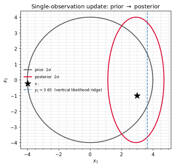

Sequential updates: $N$ factors, one addition at a time¶

Five additional measurements, each through a different $H_i$ (single coordinates and diagonal projections), each with $R = 0.5$ . The update rule is just ((2)) applied repeatedly:

\eta^{(n)} \;=\; \eta^{(n-1)} \;+\; \eta^{\rm lik}_n, \qquad \eta^{\rm lik}_n \;=\; \bigl(H_n^\top R_n^{-1} y_n,\;\; -\tfrac12\, H_n^\top R_n^{-1} H_n\bigr).

((3))

Each step is an array sum — no matrix inverses during the recursion. We only invert (via to_expectation) when we want to plot the running posterior.

H_list = [
    jnp.array([[0.0, 1.0]]),                       # y-coordinate
    jnp.array([[1.0, 1.0]]) / jnp.sqrt(2.0),       # diagonal
    jnp.array([[1.0, 0.0]]),                       # x-coordinate again
    jnp.array([[0.0, 1.0]]),                       # y-coordinate again
    jnp.array([[1.0, -1.0]]) / jnp.sqrt(2.0),      # anti-diagonal
]
R_obs = jnp.array([[0.5]])
R_obs_inv = jnp.linalg.inv(R_obs)

key = sub
ys = []
for H_i in H_list:
    key, k_obs = jax.random.split(key)
    y_i = einx.dot("k i, i -> k", H_i, x_true) \
        + jax.random.normal(k_obs, (1,)) * jnp.sqrt(R_obs[0, 0])
    ys.append(y_i)

# Recursion starting from the post-1 state.
eta1 = eta1_post1
eta2 = eta2_post1_mat

mus  = [mu0, mu1_nat]
Sigs = [Sigma0, S1_nat]

for n, (H_i, y_i) in enumerate(zip(H_list, ys, strict=True), start=2):
    eta1 = eta1 + einx.dot("k i, k l, l -> i", H_i, R_obs_inv, y_i)
    eta2 = eta2 + (-0.5) * einx.dot("k i, k l, l j -> i j", H_i, R_obs_inv, H_i)
    post_n = GaussianExpFam(eta1=eta1, eta2=psd_op(eta2))
    mu_n, S_n_op = to_expectation(post_n)
    mus.append(mu_n); Sigs.append(S_n_op.as_matrix())
    print(f"after obs {n}:  mu = [{float(mu_n[0]):+.3f}, {float(mu_n[1]):+.3f}]  "
          f"sqrt(tr Sigma) = {float(jnp.sqrt(jnp.trace(S_n_op.as_matrix()))):.3f}")

print(f"\nx_true = [{float(x_true[0]):.3f}, {float(x_true[1]):.3f}]")

after obs 2:  mu = [+2.920, -0.159]  sqrt(tr Sigma) = 1.116
after obs 3:  mu = [+2.622, -0.324]  sqrt(tr Sigma) = 0.933
after obs 4:  mu = [+2.988, -0.437]  sqrt(tr Sigma) = 0.765
after obs 5:  mu = [+3.130, -1.041]  sqrt(tr Sigma) = 0.668
after obs 6:  mu = [+2.816, -0.777]  sqrt(tr Sigma) = 0.592

x_true = [3.000, -1.000]

fig, ax = plt.subplots(figsize=(6.6, 6.0))
n_steps = len(mus)
colors  = plt.cm.viridis(np.linspace(0.1, 0.9, n_steps))
for k in range(n_steps):
    pts = ellipse_points(mus[k], Sigs[k])
    label = "prior" if k == 0 else f"after obs {k}"
    ax.plot(np.asarray(pts[0]), np.asarray(pts[1]),
            color=colors[k], lw=1.8, label=label)
    ax.scatter(float(mus[k][0]), float(mus[k][1]),
               s=22, color=colors[k], zorder=4)
ax.scatter(*np.asarray(x_true), marker="*", s=240, color="crimson",
           label=r"$x_\star$", zorder=5)
ax.set_xlabel(r"$x_1$"); ax.set_ylabel(r"$x_2$")
ax.set_title(r"Sequential Bayesian updates — $\eta$ accumulates by addition")
ax.set_aspect("equal"); ax.legend(frameon=False, fontsize=8, loc="upper left")
plt.tight_layout(); plt.show()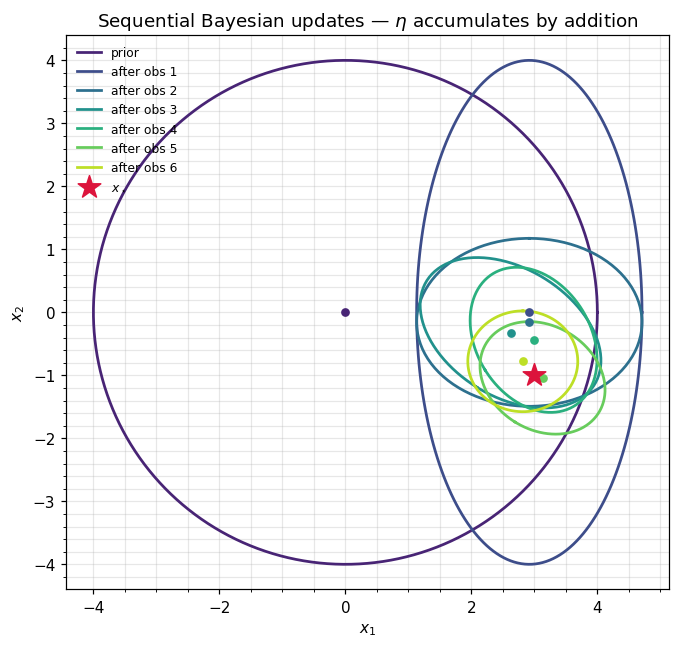

Batch = sequential = any order¶

Vector addition is commutative and associative, so the recursion ((3)) doesn’t care in what order we apply the likelihood factors:

\eta^{\rm post}_N \;=\; \eta^{\rm prior} \;+\; \sum_{i=1}^{N} \eta^{\rm lik}_i \;=\; \eta^{\rm prior} \;+\; \sum_{i=1}^{N} \eta^{\rm lik}_{\pi(i)} \quad \text{for any permutation } \pi.

((4))

This is not a coincidence of Gaussian arithmetic — it’s the defining property of exponential-family inference. Concretely:

# Stack ALL observations (including y1) and compare three computations.
H_all = [H1, *H_list]
y_all = [y1, *ys]
R_all = [R1, *([R_obs] * len(ys))]

def batch_natural(perm):
    eta1 = eta1_prior
    eta2 = eta2_prior_mat
    for j in perm:
        H, y, R = H_all[j], y_all[j], R_all[j]
        Rinv = jnp.linalg.inv(R)
        eta1 = eta1 + einx.dot("k i, k l, l -> i", H, Rinv, y)
        eta2 = eta2 + (-0.5) * einx.dot("k i, k l, l j -> i j", H, Rinv, H)
    return eta1, eta2

# (a) sequential = the order in which obs arrived
eta1_seq, eta2_seq = batch_natural(list(range(len(H_all))))
# (b) reversed
eta1_rev, eta2_rev = batch_natural(list(range(len(H_all)))[::-1])
# (c) random permutation
rng = np.random.default_rng(0)
perm = rng.permutation(len(H_all)).tolist()
eta1_rng, eta2_rng = batch_natural(perm)

ord_err_seq_rev = float(jnp.max(jnp.abs(eta1_seq - eta1_rev))) \
                + float(jnp.max(jnp.abs(eta2_seq - eta2_rev)))
ord_err_seq_rng = float(jnp.max(jnp.abs(eta1_seq - eta1_rng))) \
                + float(jnp.max(jnp.abs(eta2_seq - eta2_rng)))

# Compare to the running sequential trajectory's last entry.
last_post  = GaussianExpFam(eta1=eta1_seq, eta2=psd_op(eta2_seq))
mu_batch, S_batch_op = to_expectation(last_post)
S_batch = S_batch_op.as_matrix()

trajectory_last_mu  = mus[-1]
trajectory_last_Sig = Sigs[-1]

print(f"max ||eta(seq) - eta(reversed)||           = {ord_err_seq_rev:.2e}")
print(f"max ||eta(seq) - eta(random {perm})|| = {ord_err_seq_rng:.2e}")
print(f"max ||mu(batch)  - mu(traj last)||          = "
      f"{float(jnp.max(jnp.abs(mu_batch - trajectory_last_mu))):.2e}")
print(f"max ||Sig(batch) - Sig(traj last)||         = "
      f"{float(jnp.max(jnp.abs(S_batch - trajectory_last_Sig))):.2e}")

max ||eta(seq) - eta(reversed)||           = 1.78e-15
max ||eta(seq) - eta(random [3, 2, 5, 4, 0, 1])|| = 1.78e-15
max ||mu(batch)  - mu(traj last)||          = 0.00e+00
max ||Sig(batch) - Sig(traj last)||         = 0.00e+00

All differences sit at $\sim 10^{-15}$ — the recursion really is permutation-invariant up to round-off.

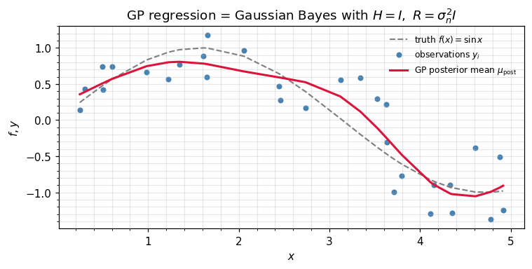
GP regression is this update¶

Gaussian-process regression with a Gaussian likelihood is precisely ((2)) applied with $H = I$ (we observe the function directly) and $R = \sigma_n^2 I$ :

\Lambda_{\rm post} \;=\; K^{-1} \;+\; \sigma_n^{-2} I, \qquad \mu_{\rm post} \;=\; \Lambda_{\rm post}^{-1}\,\sigma_n^{-2}\,y \;=\; K\,(K + \sigma_n^2 I)^{-1}\,y.

((5))

The standard GP posterior-mean formula on the right is ((5)) rearranged via the matrix-inversion identity. Different recipe, same equation.

Operationally, gaussx covers the whole loop:

N_gp = 30
key, k_x, k_y = jax.random.split(KEY, 3)
xs = jnp.sort(jax.random.uniform(k_x, (N_gp,), minval=0.0, maxval=5.0))

# RBF kernel and noisy observations of f(x) = sin(x)
ls, sigma2 = 1.0, 0.1
diff = xs[:, None] - xs[None, :]
K_gp = jnp.exp(-0.5 * diff ** 2 / ls ** 2)
f_true = jnp.sin(xs)
y_gp   = f_true + jax.random.normal(k_y, (N_gp,)) * jnp.sqrt(sigma2)

# Posterior mean: K (K + sigma^2 I)^{-1} y  -- one structured solve.
K_op = psd_op(K_gp + sigma2 * jnp.eye(N_gp))
alpha = solve(K_op, y_gp)
mu_gp = einx.dot("i j, j -> i", K_gp, alpha)

# Log marginal likelihood — used downstream for hyperparameter learning.
lml = log_marginal_likelihood(loc=jnp.zeros(N_gp), cov_operator=K_op, y=y_gp)
rmse = float(jnp.sqrt(jnp.mean((mu_gp - f_true) ** 2)))
print(f"GP log marginal likelihood : {float(lml):.3f}")
print(f"posterior-mean RMSE vs sin : {rmse:.4f}")

fig, ax = plt.subplots(figsize=(7.0, 3.6))
ax.plot(np.asarray(xs), np.asarray(f_true), "--", color="0.5",
        lw=1.4, label=r"truth $f(x) = \sin x$")
ax.scatter(np.asarray(xs), np.asarray(y_gp), s=18, color="steelblue",
           label=r"observations $y_i$")
ax.plot(np.asarray(xs), np.asarray(mu_gp), color="crimson", lw=2,
        label=r"GP posterior mean $\mu_{\rm post}$")
ax.set_xlabel(r"$x$"); ax.set_ylabel(r"$f, y$")
ax.set_title(r"GP regression = Gaussian Bayes with $H = I,\ R = \sigma_n^2 I$")
ax.legend(frameon=False, fontsize=8)
plt.tight_layout(); plt.show()

GP log marginal likelihood : -19.557
posterior-mean RMSE vs sin : 0.1561

Where this update lives in practice¶

Setting	What “factor” means	Where in the curriculum
Kalman filter (part 7)	Each observation step = one Gaussian factor folded in via ((2)). The information form is the running natural-parameter sum; the standard form is its mean-cov twin.	Information-form filter / smoother.
GP regression (part 3)	All training observations are one big factor with $H=I, R=\sigma_n^2 I$ . Posterior reduces to a single solve ((5)).	Exact, sparse, and approximate GP recipes.
Ensemble Kalman / data assimilation (part 7.x)	Each ensemble member or observation batch contributes a likelihood factor. Order-independence ((4)) lets you parallelise across sensors.	EnKF, particle Kalman, sequential 3D-Var.
EP for non-Gaussian likelihoods (part 6)	Each site approximation is a Gaussian factor in natural form. The cavity-tilted-update cycle is ((2)) with cavity = posterior − site, site = projection − cavity.	Classification GPs, robust regression.
Conjugate Bayesian linear regression	$H$ is the design matrix, $R = \sigma^2 I$ . Sequential additions handle streaming data.	Recursive least squares as a degenerate Kalman filter.
Distributed inference	Each worker computes $\eta^{\rm lik}_w$ on its shard; the parameter server sums them.	Federated GP / Bayesian linear models.

Recap¶

Linear-Gaussian Bayes rule = one application of ((5)) with the likelihood factor read off ((1)). No matrix inverses during the recursion.
$N$ observations = $N$ additions: ((3)). Mean-cov / Joseph forms are equivalent recipes if you need $(\mu, \Sigma)$ at any point.
Order-independence ((4)) is exact (modulo round-off) and is the reason exponential-family inference parallelises so cleanly.
GP regression with a Gaussian likelihood is one shot of this update ((5)), executed via gaussx.solve on the structured operator $K + \sigma_n^2 I$ .

References¶

Bernardo, J. M. & Smith, A. F. M. (2000). Bayesian Theory. Wiley.
Bishop, C. M. (2006). Pattern Recognition and Machine Learning. Springer. §2.3.
Rasmussen, C. E. & Williams, C. K. I. (2006). Gaussian Processes for Machine Learning. MIT Press. §2.2.
Minka, T. P. (2001). A family of algorithms for approximate Bayesian inference. PhD thesis, MIT.