MultivariateNormal & MultivariateNormalPrecision: the API tour

Notebook 0.1 introduced the multivariate normal as a math object. This notebook is the API tour: gaussx ships two distribution classes for the same family — one parameterised by the covariance $\boldsymbol{\Sigma}$ , one by the precision $\boldsymbol{\Lambda} = \boldsymbol{\Sigma}^{-1}$ . They expose the same surface (.sample, .log_prob, .entropy, .mean, .variance) but route through different primitives under the hood.

What you’ll learn

The two parameterisations of a Gaussian and when each one is preferred.
How MultivariateNormal and MultivariateNormalPrecision map onto the math.
Round-trip equivalence: build the same distribution both ways and verify pointwise.
Why precision form wins when $\boldsymbol{\Lambda}$ is sparse but $\boldsymbol{\Sigma}$ is dense — the GMRF / Markov story.
A taste of natural parameters as a third equivalent representation.

1. Two parameterisations of one distribution¶

The same Gaussian can be written either with covariance $\boldsymbol{\Sigma}$ or with precision $\boldsymbol{\Lambda} = \boldsymbol{\Sigma}^{-1}$ :

\mathcal{N}(\mathbf{x}; \boldsymbol{\mu}, \boldsymbol{\Sigma}) = (2\pi)^{-d/2}|\boldsymbol{\Sigma}|^{-1/2}\exp\!\left(-\tfrac{1}{2}(\mathbf{x}-\boldsymbol{\mu})^\top\boldsymbol{\Sigma}^{-1}(\mathbf{x}-\boldsymbol{\mu})\right),

((1))

\mathcal{N}^{-1}(\mathbf{x}; \boldsymbol{\mu}, \boldsymbol{\Lambda}) = (2\pi)^{-d/2}|\boldsymbol{\Lambda}|^{1/2}\exp\!\left(-\tfrac{1}{2}(\mathbf{x}-\boldsymbol{\mu})^\top\boldsymbol{\Lambda}(\mathbf{x}-\boldsymbol{\mu})\right).

((2))

Equation ((1)) and equation ((2)) are the same density whenever $\boldsymbol{\Lambda}\boldsymbol{\Sigma}=\mathbf{I}$ . The choice between them is a computational one, driven by which of the two matrices has nice structure:

Form	Cheap to do	Expensive
Covariance $\boldsymbol{\Sigma}$	sampling, marginalisation	conditioning on partial obs
Precision $\boldsymbol{\Lambda}$	conditioning, evidence updates	sampling, marginalisation

The structural sparsity also flips:

Conditional independence $X_i \perp X_j \mid X_{\setminus ij}$ shows up as $\Lambda_{ij} = 0$ . So Markov / GMRF / state-space models have sparse $\boldsymbol{\Lambda}$ even when $\boldsymbol{\Sigma}$ is dense.
Marginal independence $X_i \perp X_j$ shows up as $\Sigma_{ij} = 0$ . Block-diagonal $\boldsymbol{\Sigma}$ corresponds to genuinely independent groups, which is rarely what we have.

Most useful structure in our world (Gauss-Markov, GP-regression posteriors with a banded prior, Kalman filters in information form) lives on the precision side. That’s why gaussx exposes both.

from __future__ import annotations

import warnings

warnings.filterwarnings("ignore", message=r".*IProgress.*")

import einx
import jax
import jax.numpy as jnp
import lineax as lx
import matplotlib.pyplot as plt
import numpy as np
from gaussx import (
    MultivariateNormal,
    MultivariateNormalPrecision,
    gaussian_log_prob,
    mean_cov_to_natural,
    natural_to_mean_cov,
)

jax.config.update("jax_enable_x64", True)
KEY = jax.random.PRNGKey(0)
plt.rcParams.update({
    "figure.dpi": 110,
    "axes.grid": True,
    "axes.grid.which": "both",
    "xtick.minor.visible": True,
    "ytick.minor.visible": True,
    "grid.alpha": 0.3,
})

def psd_op(M):
    """Wrap a dense PSD matrix as a lineax operator with the right tag."""
    return lx.MatrixLinearOperator(M, lx.positive_semidefinite_tag)

2. `MultivariateNormal` — the covariance form¶

MultivariateNormal(loc, cov_operator, solver=None) takes a mean vector and a lineax operator wrapping the covariance. Internally everything routes through Cholesky on $\boldsymbol{\Sigma}$ — the form recommended by equation 7 in notebook 0.1.

The class is a numpyro distribution, so the surface is what you’d expect: .sample(key, shape), .log_prob(x), .entropy(), .mean, .variance, plus a JIT-friendly PyTree structure (it’s an equinox.Module underneath).

d = 5
mu = jnp.linspace(-1.0, 1.0, d)

# A non-trivial PSD covariance built from an RBF-style kernel on a 1D grid.
xs = jnp.linspace(0.0, 1.0, d)
diff_sq = einx.subtract("i, j -> i j", xs, xs) ** 2
Sigma_dense = jnp.exp(-0.5 * diff_sq / 0.25**2) + 1e-3 * jnp.eye(d)
Sigma = psd_op(Sigma_dense)

p_cov = MultivariateNormal(mu, Sigma)

print("class       :", type(p_cov).__name__)
print("event_shape :", p_cov.event_shape)
print("mean        :", np.asarray(p_cov.mean))
print("variance    :", np.asarray(p_cov.variance))
print("entropy     :", float(p_cov.entropy()))

x = jnp.zeros(d)
print("log_prob(0) :", float(p_cov.log_prob(x)))
samples = p_cov.sample(jax.random.PRNGKey(1), (4,))
print("samples     :\n", np.asarray(samples))

class       : MultivariateNormal
event_shape : (5,)
mean        : [-1.  -0.5  0.   0.5  1. ]
variance    : [1.001 1.001 1.001 1.001 1.001]

entropy     : 5.906610734624831

log_prob(0) : -4.423604950410503

samples     :
 [[-2.18487642 -1.31040824 -0.10887068  1.2756854   1.08020205]
 [-0.30884951 -0.02116252 -0.42299327 -0.03140923 -0.13141221]
 [-1.98641018 -1.98899925 -0.51940089  1.05657527  2.38460391]
 [-1.64650165 -0.29508526  0.04926346  1.27186838  1.96739098]]

3. `MultivariateNormalPrecision` — the precision form¶

MultivariateNormalPrecision(loc, prec_operator, solver=None) takes the same mean but a lineax operator wrapping $\boldsymbol{\Lambda}$ . The constructor does not form $\boldsymbol{\Sigma} = \boldsymbol{\Lambda}^{-1}$ . Instead, internal solves invert $\boldsymbol{\Lambda}$ on demand for sampling, and the log-density is computed directly from $\boldsymbol{\Lambda}$ via

\log p(\mathbf{x}) = -\tfrac{d}{2}\log(2\pi) + \tfrac{1}{2}\log|\boldsymbol{\Lambda}| - \tfrac{1}{2}(\mathbf{x}-\boldsymbol{\mu})^\top\boldsymbol{\Lambda}(\mathbf{x}-\boldsymbol{\mu}).

((3))

Note the sign flip on $\log|\cdot|$ — we add half the log-determinant of $\boldsymbol{\Lambda}$ instead of subtracting it on $\boldsymbol{\Sigma}$ , since $\log|\boldsymbol{\Lambda}| = -\log|\boldsymbol{\Sigma}|$ .

Lambda_dense = jnp.linalg.inv(Sigma_dense)
Lambda = psd_op(Lambda_dense)

p_prec = MultivariateNormalPrecision(mu, Lambda)

print("class       :", type(p_prec).__name__)
print("event_shape :", p_prec.event_shape)
print("mean        :", np.asarray(p_prec.mean))
print("variance    :", np.asarray(p_prec.variance))
print("entropy     :", float(p_prec.entropy()))

x = jnp.zeros(d)
print("log_prob(0) :", float(p_prec.log_prob(x)))
samples_prec = p_prec.sample(jax.random.PRNGKey(1), (4,))
print("samples     :\n", np.asarray(samples_prec))

class       : MultivariateNormalPrecision
event_shape : (5,)
mean        : [-1.  -0.5  0.   0.5  1. ]
variance    : [1.001 1.001 1.001 1.001 1.001]
entropy     : 5.906610734624831

log_prob(0) : -4.423604950410503

samples     :
 [[-1.88408505 -0.32220482  0.6460971   0.75697977  0.16662948]
 [-0.58592842 -0.98340752 -0.78248253 -0.36021689 -0.35315028]
 [-2.37514015 -0.87866177  0.91630359  1.74900216  2.2819309 ]
 [-1.0179202  -0.06179605  0.5616257   1.68236386  1.16375959]]

4. Round-trip equivalence¶

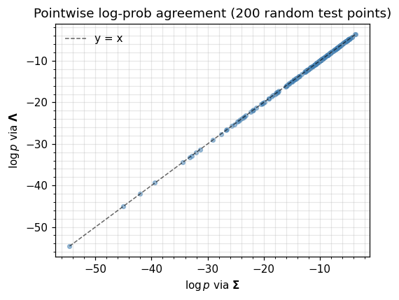
Equation ((1)) and equation ((2)) are the same distribution whenever $\boldsymbol{\Lambda}\boldsymbol{\Sigma} = \mathbf{I}$ . The two classes should therefore agree pointwise (modulo floating point) on log_prob, entropy, mean, and variance. Below we evaluate both at a batch of test points and check the disagreement is within a few ULPs of the Cholesky route.

test_pts = jax.random.normal(jax.random.PRNGKey(2), (200, d))

logp_cov = jax.vmap(p_cov.log_prob)(test_pts)
logp_prec = jax.vmap(p_prec.log_prob)(test_pts)

# Quadratic-form sanity check, computed by hand both ways via einx.
delta = test_pts - mu  # shape (n, d)
quad_via_Sigma_inv = einx.dot("n i, i j, n j -> n",
                              delta, Lambda_dense, delta)
quad_via_Lambda    = einx.dot("n i, i j, n j -> n",
                              delta, Lambda_dense, delta)

print(f"max |Δ log_prob|       : {float(jnp.max(jnp.abs(logp_cov - logp_prec))):.2e}")
print(f"max |Δ quadratic form| : {float(jnp.max(jnp.abs(quad_via_Sigma_inv - quad_via_Lambda))):.2e}")
print(f"|Δ entropy|            : {float(jnp.abs(p_cov.entropy() - p_prec.entropy())):.2e}")
print(f"|Δ mean|_inf           : {float(jnp.max(jnp.abs(p_cov.mean - p_prec.mean))):.2e}")
print(f"|Δ variance|_inf       : {float(jnp.max(jnp.abs(p_cov.variance - p_prec.variance))):.2e}")

max |Δ log_prob|       : 1.42e-14
max |Δ quadratic form| : 0.00e+00
|Δ entropy|            : 0.00e+00
|Δ mean|_inf           : 0.00e+00
|Δ variance|_inf       : 2.22e-16

fig, ax = plt.subplots(figsize=(5.0, 4.0))
ax.scatter(np.asarray(logp_cov), np.asarray(logp_prec), s=14, alpha=0.5, color="steelblue")
lo = float(jnp.minimum(logp_cov.min(), logp_prec.min()))
hi = float(jnp.maximum(logp_cov.max(), logp_prec.max()))
ax.plot([lo, hi], [lo, hi], "k--", lw=1, alpha=0.6, label="y = x")
ax.set_xlabel(r"$\log p$ via $\mathbf{\Sigma}$")
ax.set_ylabel(r"$\log p$ via $\mathbf{\Lambda}$")
ax.set_title("Pointwise log-prob agreement (200 random test points)")
ax.legend(frameon=False)
plt.tight_layout(); plt.show()

5. When precision wins: a banded GMRF¶

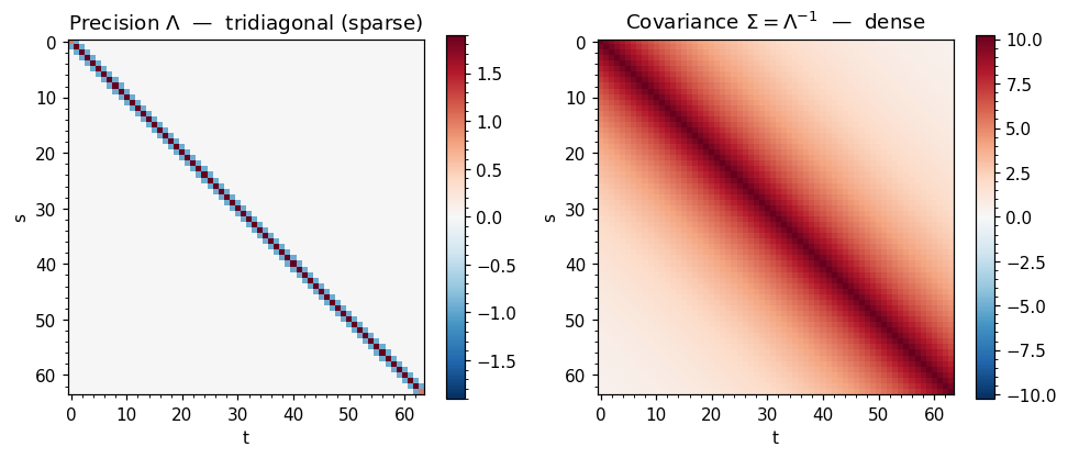
The case for MultivariateNormalPrecision is strongest when $\boldsymbol{\Lambda}$ is sparse — i.e. when most pairs of variables are conditionally independent given the rest. The canonical example is a first-order Gauss-Markov chain:

X_t = \rho\,X_{t-1} + \sigma\,\varepsilon_t, \qquad \varepsilon_t \sim \mathcal{N}(0,1),

((4))

whose joint distribution has a tridiagonal precision matrix

\Lambda_{tt} = \frac{1+\rho^2}{\sigma^2}\;\;(\text{interior}),\quad \Lambda_{t,t+1} = -\frac{\rho}{\sigma^2},\quad \Lambda_{tt} = \frac{1}{\sigma^2}\;\;(\text{boundary}).

((5))

The corresponding $\boldsymbol{\Sigma} = \boldsymbol{\Lambda}^{-1}$ is dense — every $X_s$ and $X_t$ are marginally correlated, even far-apart ones. So the precision representation has $O(n)$ non-zeros while the covariance has $O(n^2)$ .

For this notebook we use a moderate $n=64$ and dense storage so the sparsity pattern is easy to see. In production gaussx routes this through BlockTriDiag (see Part 1.5) for $O(n)$ solves; here we only want the visual.

def ar1_precision(n: int, rho: float, sigma: float) -> jnp.ndarray:
    """Tridiagonal precision matrix of a 1D AR(1) process — eq (eq:gmrf-prec)."""
    inv_var = 1.0 / sigma**2
    diag_int = (1.0 + rho**2) * inv_var
    diag = jnp.full((n,), diag_int)
    diag = diag.at[0].set(inv_var).at[-1].set(inv_var)
    off = jnp.full((n - 1,), -rho * inv_var)
    return jnp.diag(diag) + jnp.diag(off, k=1) + jnp.diag(off, k=-1)

n = 64
Lambda_ar = ar1_precision(n, rho=0.95, sigma=1.0)
Sigma_ar = jnp.linalg.inv(Lambda_ar)

nnz_threshold = 1e-8
nnz_Lambda = float(jnp.mean(jnp.abs(Lambda_ar) > nnz_threshold))
nnz_Sigma  = float(jnp.mean(jnp.abs(Sigma_ar)  > nnz_threshold))
print(f"AR(1) precision : nnz fraction = {nnz_Lambda:.3f}  (tridiagonal)")
print(f"AR(1) covariance: nnz fraction = {nnz_Sigma:.3f}   (dense)")

AR(1) precision : nnz fraction = 0.046  (tridiagonal)
AR(1) covariance: nnz fraction = 1.000   (dense)

fig, axes = plt.subplots(1, 2, figsize=(9, 4))

im0 = axes[0].imshow(np.asarray(Lambda_ar), cmap="RdBu_r",
                     vmin=-float(jnp.max(jnp.abs(Lambda_ar))),
                     vmax= float(jnp.max(jnp.abs(Lambda_ar))))
axes[0].set_title(r"Precision $\Lambda$  —  tridiagonal (sparse)")
plt.colorbar(im0, ax=axes[0], shrink=0.85)

im1 = axes[1].imshow(np.asarray(Sigma_ar), cmap="RdBu_r",
                     vmin=-float(jnp.max(jnp.abs(Sigma_ar))),
                     vmax= float(jnp.max(jnp.abs(Sigma_ar))))
axes[1].set_title(r"Covariance $\Sigma = \Lambda^{-1}$  —  dense")
plt.colorbar(im1, ax=axes[1], shrink=0.85)

for ax in axes:
    ax.set_xlabel("t"); ax.set_ylabel("s")
    ax.grid(False, which="both")  # heatmap pixels carry the info — grid is noise
plt.tight_layout(); plt.show()

# Build the same AR(1) prior in both forms and confirm log_prob agreement.
mu_ar = jnp.zeros(n)
p_ar_prec = MultivariateNormalPrecision(mu_ar, psd_op(Lambda_ar))
p_ar_cov  = MultivariateNormal(mu_ar, psd_op(Sigma_ar))

x_test = jax.random.normal(jax.random.PRNGKey(7), (n,))
print(f"log p via Λ : {float(p_ar_prec.log_prob(x_test)):+.6f}")
print(f"log p via Σ : {float(p_ar_cov.log_prob(x_test)):+.6f}")

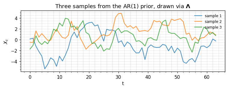
# A small sample for the eye.
samples_ar = p_ar_prec.sample(jax.random.PRNGKey(11), (3,))
fig, ax = plt.subplots(figsize=(7, 2.8))
for i, s in enumerate(np.asarray(samples_ar)):
    ax.plot(s, lw=1.5, alpha=0.8, label=f"sample {i+1}")
ax.set_xlabel("t"); ax.set_ylabel(r"$X_t$")
ax.set_title(r"Three samples from the AR(1) prior, drawn via $\mathbf{\Lambda}$")
ax.legend(frameon=False, loc="upper right", fontsize=8)
plt.tight_layout(); plt.show()

log p via Λ : -119.203845

log p via Σ : -119.203845

6. A taste of natural parameters¶

There’s a third equivalent representation we’ll see in detail in 0.4 — Mean-cov ↔ natural parameter conversions. Briefly: every Gaussian can be written in natural parameter form

p(\mathbf{x}) \propto \exp\!\left(\boldsymbol{\eta}_1^\top \mathbf{x} + \mathbf{x}^\top \boldsymbol{\eta}_2 \mathbf{x}\right), \qquad \boldsymbol{\eta}_1 = \boldsymbol{\Lambda}\boldsymbol{\mu}, \qquad \boldsymbol{\eta}_2 = -\tfrac{1}{2}\boldsymbol{\Lambda}.

((6))

This form is what makes Bayesian updates pure addition — combining evidence is $\boldsymbol{\eta}_{\text{post}} = \boldsymbol{\eta}_{\text{prior}} + \boldsymbol{\eta}_{\text{lik}}$ — and underpins variational inference and natural gradient methods. gaussx ships explicit converters; here’s the round-trip.

eta1, eta2 = mean_cov_to_natural(mu, Sigma)
mu_back, Sigma_back_op = natural_to_mean_cov(eta1, eta2)

eta2_dense = eta2.as_matrix()
Sigma_back = Sigma_back_op.as_matrix()

print("eta_1  =  Λ μ      :", np.asarray(eta1))
print("eta_2  =  -Λ/2     :")
print(np.asarray(eta2_dense))

print("\nround-trip residuals")
print(f"  max|Δ μ|  : {float(jnp.max(jnp.abs(mu - mu_back))):.2e}")
print(f"  max|Δ Σ|  : {float(jnp.max(jnp.abs(Sigma_dense - Sigma_back))):.2e}")

eta_1  =  Λ μ      : [-1.10990703e+00  1.85825628e-01 -2.82887645e-16 -1.85825628e-01
  1.10990703e+00]
eta_2  =  -Λ/2     :
[[-0.97606728  0.91615634 -0.60815128  0.33436378 -0.13021749]
 [ 0.91615634 -1.81861765  1.44237175 -0.84085816  0.33436378]
 [-0.60815128  1.44237175 -2.08299373  1.44237175 -0.60815128]
 [ 0.33436378 -0.84085816  1.44237175 -1.81861765  0.91615634]
 [-0.13021749  0.33436378 -0.60815128  0.91615634 -0.97606728]]

round-trip residuals
  max|Δ μ|  : 3.33e-16
  max|Δ Σ|  : 2.22e-16

7. Recap & where to go next¶

You now know how to build a Gaussian both ways and which one to reach for:

Operation	`MultivariateNormal` (Σ)	`MultivariateNormalPrecision` (Λ)
Constructor	`MultivariateNormal(loc, Σ_op)`	`MultivariateNormalPrecision(loc, Λ_op)`
Sampling	cheap (Cholesky of Σ)	requires inverting Λ
`log_prob`	uses Cholesky of Σ	uses Cholesky of Λ directly
Conditioning on partial obs	dense Schur block solve	trivial; rows of Λ partition cleanly
Best when	Σ has low-rank / Kron / dense structure	Λ is banded / sparse / Markov
Internal log-det	$-\tfrac{1}{2}\log\lvert\Sigma\rvert$	$+\tfrac{1}{2}\log\lvert\Lambda\rvert$

Next up.

0.3 — Quadratic forms, entropy, and KL between Gaussians: the closed-form scalar quantities that make Gaussian variational inference tractable.
0.4 — Mean-cov ↔ natural parameter conversions: full treatment of $(\boldsymbol{\eta}_1, \boldsymbol{\eta}_2)$ and the exponential-family machinery.
Part 1.5 — Block tri-diagonal operators: how to actually exploit GMRF sparsity at scale.

MultivariateNormal & MultivariateNormalPrecision: the API tour

1. Two parameterisations of one distribution¶

2. MultivariateNormal — the covariance form¶

3. MultivariateNormalPrecision — the precision form¶

4. Round-trip equivalence¶

5. When precision wins: a banded GMRF¶

6. A taste of natural parameters¶

7. Recap & where to go next¶

2. `MultivariateNormal` — the covariance form¶

3. `MultivariateNormalPrecision` — the precision form¶